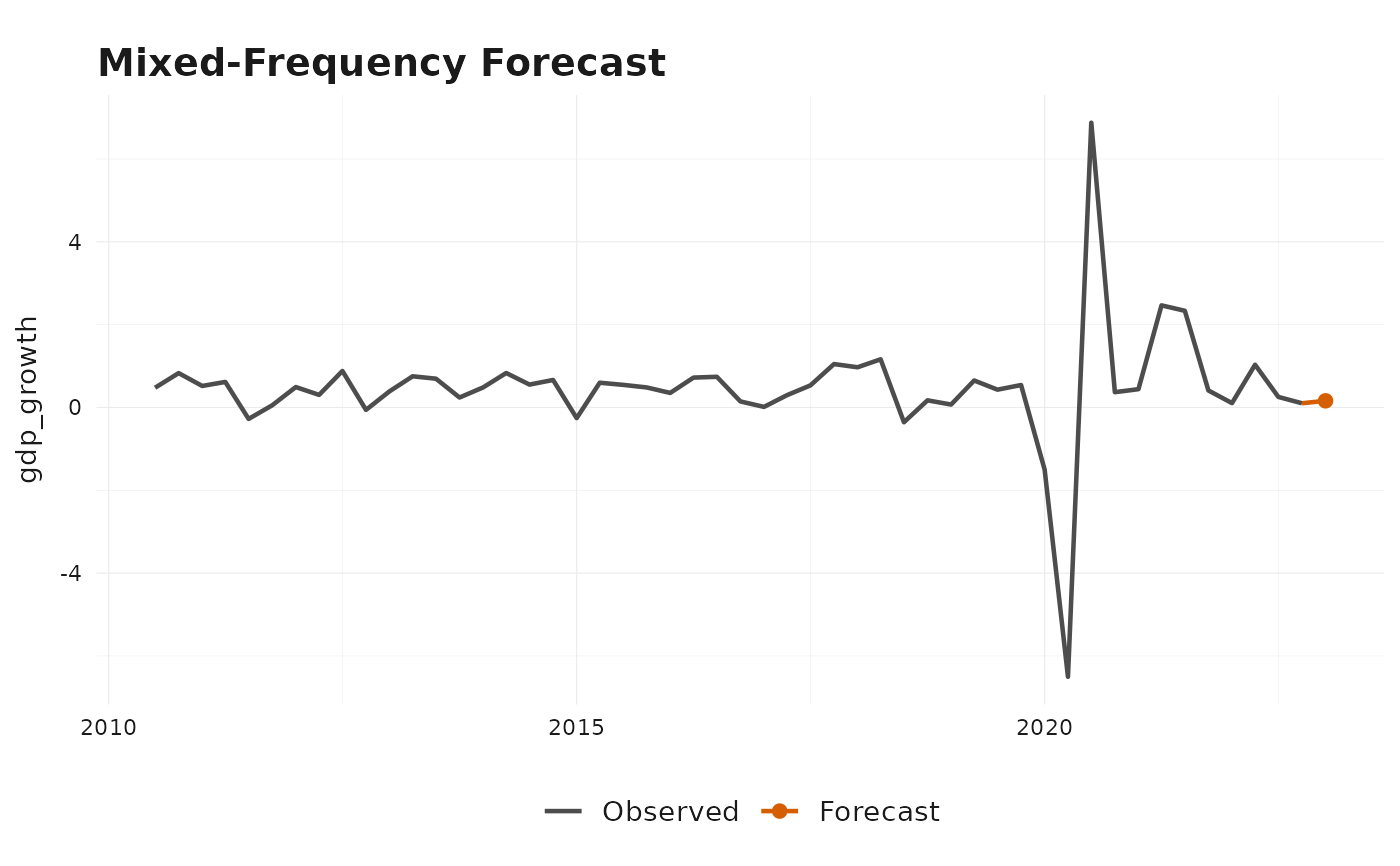
Plot a Mixed-Frequency Forecast — plot.mf_model

Visualize a "mf_model_forecast" object returned by forecast.mf_model(), showing the observed target history together with the bridge forecast and, when available, a prediction interval.

Usage

# S3 method for class 'mf_model_forecast'
plot(
  x,
  level = NULL,
  history_n = 50,
  xlab = NULL,
  ylab = NULL,
  main = NULL,
  ...
)

# S3 method for class 'mf_model_forecast'
autoplot(object, ...)

Arguments

x: A "mf_model_forecast" object returned by forecast.mf_model().
level: Prediction interval level to display. Must be one of the levels the forecast was computed with. Defaults to the first available level.
history_n: Number of historical target observations to display. Defaults to the most recent 50. Set to NULL to show the full history.
xlab, ylab, main: Optional axis and title labels.
...: Additional arguments passed to theme_bridgr().
object: A "mf_model_forecast" object, for the ggplot2::autoplot() method.

Value

A ggplot2 object.

Details

These methods are provided directly for "mf_model_forecast" rather than inherited from the forecast package, so that plotting works for every target frequency mf_model() supports, including daily and weekly targets that stats::ts() cannot represent. See as.forecast() to convert to a "forecast" object where the frequency allows it.

Examples

gdp_growth <- tsbox::ts_pc(gdp)
#> [value]: 'values' 
#> [value]: 'values' 
gdp_growth <- tsbox::ts_na_omit(gdp_growth)
#> [value]: 'values' 
model <- mf_model(
  target = gdp_growth,
  indic = baro,
  indic_predict = "auto.arima",
  indic_aggregators = "mean",
  h = 1
)

plot(forecast(model))