Overview
bridgr covers classic bridge equations, MIDAS-style
mixed-frequency regressions, and intermediate specifications that
estimate within-period weights from the data, all behind a single
workflow for bridging high-frequency indicators to a
lower-frequency target.
The core workflow is always the same:
- Provide one lower-frequency target series and one or more higher-frequency indicators.
- Decide how missing indicator observations should be handled with
indic_predict. - Decide how indicators should be aligned to the target frequency with
indic_aggregators. - Fit the target equation with
mf_model(), inspect it withsummary(), and produce target-period forecasts withforecast().
This vignette walks through that workflow with the package’s built-in Swiss GDP and indicator data.
Example Data
gdp_growth <- suppressMessages(tsbox::ts_na_omit(tsbox::ts_pc(gdp)))

head(gdp_growth)
#> # A tibble: 6 × 2
#>   time       values
#>   <date>      <dbl>
#> 1 2004-04-01  0.839
#> 2 2004-07-01 -0.104
#> 3 2004-10-01  0.242
#> 4 2005-01-01  0.860
#> 5 2005-04-01  1.06
#> 6 2005-07-01  1.15
head(baro)
#> # A tibble: 6 × 2
#>   time       values
#>   <date>      <dbl>
#> 1 2004-01-01   109.
#> 2 2004-02-01   108.
#> 3 2004-03-01   109.
#> 4 2004-04-01   110.
#> 5 2004-05-01   109.
#> 6 2004-06-01   105.
gdp_growth is quarterly, while baro is
monthly. mf_model() recognizes the frequency mismatch
automatically and aligns the indicator to the target frequency before
fitting the target equation.
Stationarity expectations
bridgr assumes that the series you submit are already on
a scale that is suitable for linear regression — typically growth rates,
differences, or similarly stabilized transformations. The package does
not automatically re-transform inputs, but you can enable a lightweight
pre-fit diagnostic through stationarity = "warn". The
example below shows the warning on a level GDP series and confirms that
it disappears after differencing to growth rates.
gdp_level_recent <- dplyr::slice_tail(gdp, n = 40)
baro_recent <- dplyr::slice_tail(baro, n = 120)

invisible(tryCatch(
  mf_model(
    target = gdp_level_recent,
    indic = baro_recent,
    indic_predict = "last",
    indic_aggregators = "mean",
    h = 1,
    stationarity = "warn"
  ),
  warning = function(w) message("Warning captured: ", conditionMessage(w))
))
#> Warning captured: Heuristic stationarity checks flagged target series `gdp_level_recent` (KPSS differencing signal). Consider differences, growth rates, log changes, demeaning, or other variance-stabilizing transformations before fitting.

stationary_model <- mf_model(
  target = gdp_growth,
  indic = baro,
  indic_predict = "last",
  indic_aggregators = "mean",
  h = 1,
  stationarity = "warn"
)
A Basic Bridge Model
bridge_model <- mf_model(
  target = gdp_growth,
  indic = baro,
  indic_predict = "auto.arima",
  indic_aggregators = "mean",
  indic_lags = 1,
  target_lags = 1,
  h = 2
)

forecast(bridge_model)
#> Mixed-frequency forecast
#> -----------------------------------
#> Target series: gdp_growth
#> Forecast horizon: 2
#> Uncertainty: point forecast only
#> -----------------------------------
#>   time       mean
#> 1 2023-01-01 0.875
#> 2 2023-04-01 0.678
The default "mean" aggregator is the classic
bridge-model setup: each monthly block is completed first, then averaged
to the quarterly frequency before the target equation is estimated.
The fitted object stores the aligned data that went into estimation and the future target-period regressor path used for forecasting.
tail(bridge_model$estimation_set)
#> # A tibble: 6 × 5
#>   time       gdp_growth  baro baro_lag1 gdp_growth_lag1
#>   <date>          <dbl> <dbl>     <dbl>           <dbl>
#> 1 2021-07-01      2.34  112.      125.            2.47
#> 2 2021-10-01      0.411 104.      112.            2.34
#> 3 2022-01-01      0.105  97.4     104.            0.411
#> 4 2022-04-01      1.03   94.3      97.4           0.105
#> 5 2022-07-01      0.255  90.0      94.3           1.03
#> 6 2022-10-01      0.102  90.7      90.0           0.255
bridge_model$forecast_set
#> # A tibble: 2 × 4
#>   time        baro baro_lag1 gdp_growth_lag1
#>   <date>     <dbl>     <dbl> <list>
#> 1 2023-01-01  97.4      90.7 <dbl [1]>
#> 2 2023-04-01  99.8      97.4 <dbl [1]>
Lags in the target equation
target_lags = p adds p autoregressive lags
of the target to the right-hand side of the regression.
indic_lags = q adds q lags of each
aggregated indicator (after frequency alignment). Both default to
0. In the example above the target equation is
\[ \Delta y_t = \alpha + \rho \, \Delta y_{t-1} + \beta_0 \, \bar{x}_t + \beta_1 \, \bar{x}_{t-1} + \varepsilon_t, \]
where \(\bar{x}_t\) is the within-quarter mean of the monthly indicator. Forecasts beyond the first horizon are produced recursively, with simulated target lags taking the place of observed ones once the in-sample history is exhausted.
Standardized Output
summary() and forecast() use a stable
package-specific layout. The base output is the same across bridge,
mixed-frequency, and direct-alignment specifications. Additional
details, such as optimization summaries or uncertainty settings, are
appended only when they are relevant.
summary(bridge_model)
#> Mixed-frequency model summary
#> -----------------------------------
#> Target series: gdp_growth
#> Target frequency: quarter
#> Forecast horizon: 2
#> Estimation rows: 73
#> Regressors: baro, baro_lag1, gdp_growth_lag1
#> -----------------------------------
#> Target equation coefficients:
#>                 Estimate
#> (Intercept)       -6.249
#> baro               0.151
#> baro_lag1         -0.084
#> gdp_growth_lag1    0.012
#> -----------------------------------
#> Model fit:
#>  Statistic               Value
#>  R-squared               0.682
#>  Adjusted R-squared      0.668
#>  Residual standard error 0.773
#> -----------------------------------
#> Indicator summary:
#>      Frequency Predict    Aggregation
#> baro month     auto.arima mean
#> -----------------------------------
Forecast Visualization
The package also provides a built-in plotting method for fitted
mixed-frequency models. With type = "forecast", it shows
the observed target history together with the forecast path generated by
the model.
plot(bridge_model, type = "forecast")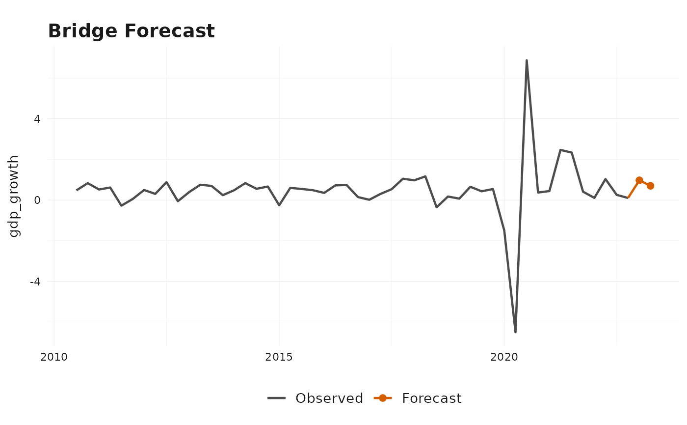
Multiple Indicators
mf_model() accepts any number of indicators in a single
long-format table. Indicators may share a frequency or come from
different frequencies, in which case each one is aligned to the target
separately. The example below pairs the level of the KOF barometer with
its year-over-year change as two monthly indicators.
baro_yoy <- baro |>
  dplyr::arrange(time) |>
  dplyr::mutate(values = values - dplyr::lag(values, 12)) |>
  dplyr::filter(!is.na(values))

indic_multi <- dplyr::bind_rows(
  dplyr::mutate(baro, id = "baro_level"),
  dplyr::mutate(baro_yoy, id = "baro_yoy")
) |>
  dplyr::select(id, time, values)

multi_model <- mf_model(
  target = gdp_growth,
  indic = indic_multi,
  indic_predict = c("last", "last"),
  indic_aggregators = c("mean", "mean"),
  target_lags = 1,
  h = 1
)

multi_model$regressor_names
#> [1] "baro_level"      "baro_yoy"        "gdp_growth_lag1"
forecast(multi_model)
#> Mixed-frequency forecast
#> -----------------------------------
#> Target series: gdp_growth
#> Forecast horizon: 1
#> Uncertainty: point forecast only
#> -----------------------------------
#>   time       mean
#> 1 2023-01-01 -0.324
Both indicators are aggregated independently and enter the final target equation as separate regressors.
Direct Alignment
If you set indic_predict = "direct", bridgr
switches from indicator forecasting to direct alignment based only on
observed complete high-frequency blocks. In that case, the latest
complete blocks are assigned backward to target periods instead of being
forecast forward first, and they are averaged within each target
period.
direct_model <- mf_model(
  target = gdp_growth,
  indic = baro,
  indic_predict = "direct",
  h = 1
)

forecast(direct_model)
#> Mixed-frequency forecast
#> -----------------------------------
#> Target series: gdp_growth
#> Forecast horizon: 1
#> Uncertainty: point forecast only
#> -----------------------------------
#>   time       mean
#> 1 2023-01-01 -0.497
This is particularly useful at the ragged edge when you want to work only with observed high-frequency information and avoid a separate indicator forecasting step.
Non-Standard Calendars
By default the package uses a regular frequency ladder
(second → minute → hour →
day → week → month →
quarter → year) with conventional conversion
factors such as 60 seconds per minute, 24 hours per day, and 3 months
per quarter. If your data follow a non-standard calendar — for example a
5-day business week or 50 working weeks per year — pass a named numeric
vector to frequency_conversions to override the defaults.
See ?mf_model for the full set of recognized names.
Optional Uncertainty Output
By default, bridgr returns point forecasts only. If you
want uncertainty output, request it at estimation time with
se = TRUE and, if needed, custom simulation or full-system
bootstrap controls through bootstrap.
uncertainty_model <- mf_model(
  target = gdp_growth,
  indic = baro,
  indic_predict = "auto.arima",
  indic_aggregators = "mean",
  target_lags = 1,
  h = 4,
  se = TRUE,
  bootstrap = list(N = 40, block_length = NULL)
)

forecast(uncertainty_model)
#> Mixed-frequency forecast
#> -----------------------------------
#> Target series: gdp_growth
#> Forecast horizon: 4
#> Uncertainty: prediction intervals from residual resampling
#> Simulation paths: 40
#> -----------------------------------
#>   time       mean  se    lower_80 upper_80 lower_95 upper_95
#> 1 2023-01-01 0.259 0.742 -0.804   0.975    -1.085   2.423
#> 2 2023-04-01 0.486 0.788 -0.593   1.750    -0.891   1.939
#> 3 2023-07-01 0.500 0.784 -0.601   1.422    -0.961   2.522
#> 4 2023-10-01 0.521 0.865 -0.579   1.626    -0.838   2.742
summary(uncertainty_model)
#> Mixed-frequency model summary
#> -----------------------------------
#> Target series: gdp_growth
#> Target frequency: quarter
#> Forecast horizon: 4
#> Estimation rows: 74
#> Regressors: baro, gdp_growth_lag1
#> -----------------------------------
#> Target equation coefficients:
#>                 Estimate HAC SE
#> (Intercept)      -10.988  3.304
#> baro               0.116  0.033
#> gdp_growth_lag1   -0.316  0.120
#> -----------------------------------
#> Model fit:
#>  Statistic               Value
#>  R-squared               0.572
#>  Adjusted R-squared      0.560
#>  Residual standard error 0.886
#> -----------------------------------
#> Indicator summary:
#>      Frequency Predict    Aggregation
#> baro month     auto.arima mean
#> -----------------------------------
#> Uncertainty:
#> Coefficient SEs: hac
#> Prediction intervals: residual resampling
#> Simulation paths: 40
#> -----------------------------------
plot(uncertainty_model, type = "forecast")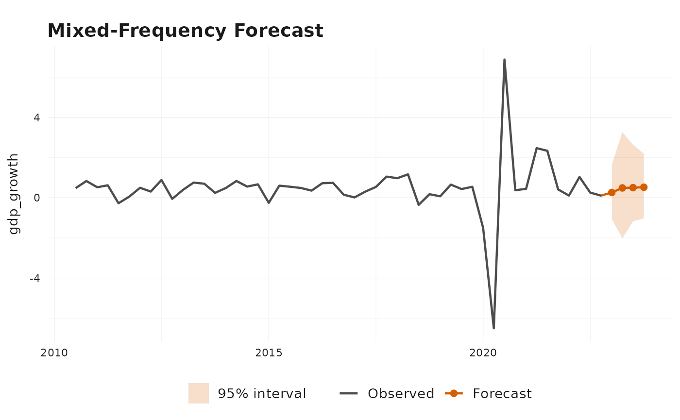
The uncertainty implementation uses HAC standard errors for the
linear target equation, or Delta-HAC standard errors when parametric
aggregation weights are estimated jointly. By default, prediction
intervals are simulated from resampled centered target-equation
residuals. If you also set full_system_bootstrap = TRUE,
bridgr instead uses a full-system target-period block
bootstrap for both coefficient standard errors and prediction intervals,
controlled through
bootstrap = list(N = ..., block_length = ...).
Where to Go Next
The vignette
vignette("mixed-frequency-modeling", package = "bridgr")
compares the main aggregation strategies and shows how
bridgr moves from classic bridge models to unrestricted and
parametric MIDAS-style specifications.
The vignette
vignette("ragged-edge-nowcasting", package = "bridgr")
focuses on indic_predict and the different ways to handle
incomplete high-frequency data at the forecast origin.
The vignette
vignette("uncertainty-and-scenarios", package = "bridgr")
shows how to work with HAC / Delta-HAC coefficient uncertainty,
residual-resampling prediction intervals, the optional full-system
bootstrap, and scenario forecasts based on custom future regressor
paths.