Aggregation and Mixed-Frequency Modeling in bridgr

The Bridge-to-MIDAS Spectrum

The key design choice in bridgr is that classic bridge equations, unrestricted mixed-frequency regressions, and parametric MIDAS-style models all share the same estimation, forecasting, and summary workflow. You can move between them without switching to a different API.

bridgr supports several ways to map higher-frequency observations into a lower-frequency target equation. Those choices span a continuum:

Bridge-style deterministic aggregation: "mean", "last", "sum", or a fixed numeric weight vector.
Unrestricted mixed-frequency regression: "unrestricted".
Parametric MIDAS-style weighting: "expalmon" and "beta".

This vignette uses a simple monthly-to-quarterly simulation so the differences between these approaches are easy to see.

A Small Monthly-to-Quarterly Example

n_quarters <- 40
quarter_index <- rep(seq_len(n_quarters), each = 3)
slot <- rep(1:3, times = n_quarters)
monthly_time <- seq(
  as.Date("2010-01-01"),
  by = "month",
  length.out = n_quarters * 3
)
monthly_indicator <- dplyr::tibble(
  time = monthly_time,
  value = 15 + quarter_index * 0.35 +
    ifelse(slot == 1, 0.8 * sin(quarter_index / 2), 0) +
    ifelse(slot == 2, -0.6 * cos(quarter_index / 3), 0) +
    ifelse(slot == 3, 0.7 * sin(quarter_index / 4 + 0.3), 0)
)

quarter_time <- monthly_time[seq(1, length(monthly_time), by = 3)]
quarter_target <- dplyr::tibble(
  time = quarter_time,
  value = 0.5 +
    vapply(
      seq_along(quarter_time),
      function(i) {
        block <- monthly_indicator$value[((i - 1) * 3 + 1):(i * 3)]
        0.2 * block[[1]] + 0.6 * block[[2]] + 0.2 * block[[3]]
      },
      numeric(1)
    ) +
    rep(c(0.1, -0.05, 0.08, -0.02), length.out = length(quarter_time))
)

The data-generating process is intentionally driven more by the middle month of each quarter — the within-quarter weights are (0.2, 0.6, 0.2) — so we can see how the different aggregation schemes react. The monthly indicator also has slot-specific within-quarter movements, so the unrestricted specification can estimate three distinct monthly coefficients.

Deterministic Bridge Aggregation

mean_model <- mf_model(
  target = quarter_target,
  indic = monthly_indicator,
  indic_predict = "last",
  indic_aggregators = "mean",
  h = 1
)

last_model <- mf_model(
  target = quarter_target,
  indic = monthly_indicator,
  indic_predict = "last",
  indic_aggregators = "last",
  h = 1
)

summary(mean_model)
#> Mixed-frequency model summary
#> -----------------------------------
#> Target series: quarter_target
#> Target frequency: quarter
#> Forecast horizon: 1
#> Estimation rows: 40
#> Regressors: monthly_indicator
#> -----------------------------------
#> Target equation coefficients:
#>                   Estimate
#> (Intercept)          0.516
#> monthly_indicator    0.999
#> -----------------------------------
#> Model fit:
#>  Statistic               Value
#>  R-squared               0.999
#>  Adjusted R-squared      0.999
#>  Residual standard error 0.142
#> -----------------------------------
#> Indicator summary:
#>                   Frequency Predict Aggregation
#> monthly_indicator month     last    mean       
#> -----------------------------------

These are classic bridge-model choices. They are easy to interpret and often work well when you want a transparent rule for within-period aggregation.

Fixed numeric weights

If you already have a prior about the within-period shape, pass a numeric weight vector in a list() instead. Weights must have the right length for the inferred target-period block size and must sum to one.

fixed_model <- mf_model(
  target = quarter_target,
  indic = monthly_indicator,
  indic_predict = "last",
  indic_aggregators = list(c(0.1, 0.7, 0.2)),
  h = 1
)

stats::coef(fixed_model)
#>       (Intercept) monthly_indicator 
#>         0.5676102         0.9984672

Unrestricted Mixed-Frequency Regression

unrestricted_model <- mf_model(
  target = quarter_target,
  indic = monthly_indicator,
  indic_predict = "last",
  indic_aggregators = "unrestricted",
  h = 1
)

stats::coef(unrestricted_model)
#>           (Intercept) monthly_indicator_hf1 monthly_indicator_hf2 
#>             0.5411254             0.1983962             0.5961748 
#> monthly_indicator_hf3 
#>             0.2047900

"unrestricted" estimates one coefficient for each within-quarter monthly observation. In a monthly-on-quarterly example this means three separate regressors. Notice that the recovered coefficients are close to the true (0.2, 0.6, 0.2) weights used in the simulated DGP — the second slot dominates, as designed.

This example keeps indic_predict = "last" so the comparison isolates the aggregation choice. The ragged-edge vignette covers indic_predict = "direct", which skips indicator forecasting and instead works from the latest observed complete high-frequency blocks.

Parametric MIDAS-Style Weighting

bridgr also supports parametric weighting rules that estimate the within-period shape from the data while keeping the number of free parameters small. The solver_options list controls the optimizer — see ?mf_model for the full set of available controls.

expalmon_model <- mf_model(
  target = quarter_target,
  indic = monthly_indicator,
  indic_predict = "last",
  indic_aggregators = "expalmon",
  solver_options = list(seed = 123, n_starts = 1, maxiter = 100),
  h = 1
)

beta_model <- mf_model(
  target = quarter_target,
  indic = monthly_indicator,
  indic_predict = "last",
  indic_aggregators = "beta",
  solver_options = list(
    seed = 123,
    n_starts = 1,
    maxiter = 100,
    start_values = c(2, 2)
  ),
  h = 1
)

The fitted object stores both the estimated weight profile and the underlying parametric coefficients.

indicator_id <- expalmon_model$indic_name[[1]]

equal_weights <- rep(1 / 3, 3)
last_weights <- c(0, 0, 1)
true_weights <- c(0.2, 0.6, 0.2)

weights_df <- dplyr::bind_rows(
  dplyr::tibble(model = "mean",        month = 1:3, weight = equal_weights),
  dplyr::tibble(model = "last",        month = 1:3, weight = last_weights),
  dplyr::tibble(model = "true DGP",    month = 1:3, weight = true_weights),
  dplyr::tibble(model = "expalmon",    month = 1:3,
                weight = expalmon_model$parametric_weights[[indicator_id]]),
  dplyr::tibble(model = "beta",        month = 1:3,
                weight = beta_model$parametric_weights[[indicator_id]])
)

ggplot2::ggplot(
  weights_df,
  ggplot2::aes(x = .data$month, y = .data$weight, color = .data$model)
) +
  ggplot2::geom_line(linewidth = 0.8) +
  ggplot2::geom_point(size = 2) +
  ggplot2::scale_x_continuous(breaks = 1:3) +
  ggplot2::labs(
    title = "Within-quarter weight profiles",
    x = "Month within quarter",
    y = "Weight"
  ) +
  theme_bridgr()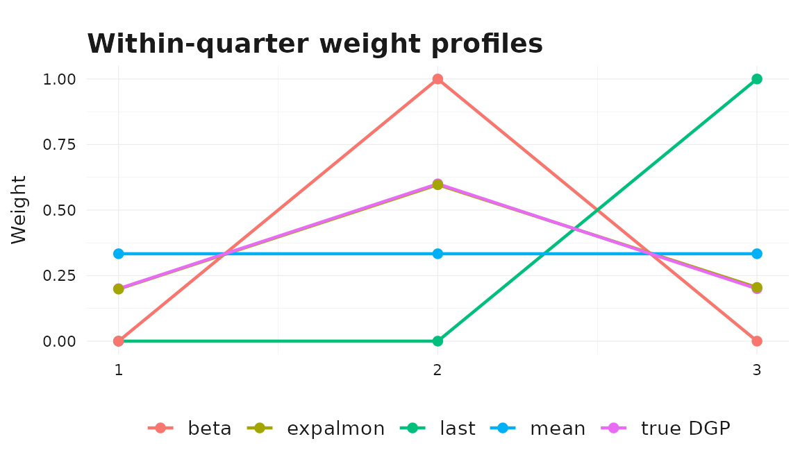

The parametric profiles concentrate mass on the middle month, matching the simulated DGP. The fixed "mean" rule spreads mass evenly across months and "last" puts all of it on the final month.

Forecast Comparison

All of these models share the same downstream interface.

forecasts_df <- dplyr::bind_rows(
  dplyr::tibble(model = "mean",
                forecast = as.numeric(forecast(mean_model)$mean)),
  dplyr::tibble(model = "last",
                forecast = as.numeric(forecast(last_model)$mean)),
  dplyr::tibble(model = "unrestricted",
                forecast = as.numeric(forecast(unrestricted_model)$mean)),
  dplyr::tibble(model = "expalmon",
                forecast = as.numeric(forecast(expalmon_model)$mean)),
  dplyr::tibble(model = "beta",
                forecast = as.numeric(forecast(beta_model)$mean))
)

ggplot2::ggplot(
  forecasts_df,
  ggplot2::aes(x = .data$model, y = .data$forecast, fill = .data$model)
) +
  ggplot2::geom_col(width = 0.6, show.legend = FALSE) +
  ggplot2::labs(
    title = "One-step-ahead forecast by aggregation strategy",
    x = NULL, y = "Forecast"
  ) +
  theme_bridgr()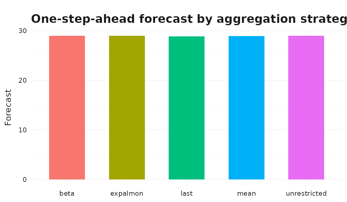

Picking an Aggregator on Out-of-Sample Performance

A rough rule-of-thumb guide to aggregator choice is given at the end of this vignette. In practice the best way to choose is to evaluate candidate models on out-of-sample forecasts. The example below uses a short pseudo-real-time rolling-origin scheme on the simulated data, with one-quarter-ahead forecasts.

origins <- (n_quarters - 13):(n_quarters - 4)
methods <- c("mean", "unrestricted", "expalmon")

eval_rows <- list()
for (m in methods) {
  for (origin in origins) {
    train <- dplyr::slice(quarter_target, seq_len(origin))
    truth <- quarter_target$value[[origin + 1]]
    fit <- mf_model(
      target = train,
      indic = monthly_indicator,
      indic_predict = "last",
      indic_aggregators = m,
      h = 1,
      solver_options = if (m == "expalmon") {
        list(seed = 1, n_starts = 1, maxiter = 100)
      } else {
        NULL
      }
    )
    fc <- as.numeric(forecast(fit)$mean)[[1]]
    eval_rows[[length(eval_rows) + 1]] <- dplyr::tibble(
      method = m, origin = origin, forecast = fc, actual = truth
    )
  }
}

eval_df <- dplyr::bind_rows(eval_rows)
eval_summary <- eval_df |>
  dplyr::group_by(.data$method) |>
  dplyr::summarise(
    rmse = sqrt(mean((.data$forecast - .data$actual)^2)),
    mae = mean(abs(.data$forecast - .data$actual)),
    .groups = "drop"
  )

eval_summary
#> # A tibble: 3 × 3
#>   method         rmse    mae
#>   <chr>         <dbl>  <dbl>
#> 1 expalmon     0.0701 0.0686
#> 2 mean         0.107  0.0870
#> 3 unrestricted 0.0701 0.0686

Even on this small example the unrestricted and parametric specifications recover the within-quarter shape and outperform the deterministic mean. For a real application you would typically use a longer evaluation window, multiple horizons, and richer scoring rules.

Choosing an Aggregation Strategy

As a rough guide:

Use deterministic bridge aggregation like "mean", "last", or "sum" when you want a transparent and stable nowcasting rule.
Use "unrestricted" when the frequency gap is small and you want each within-period observation to have its own coefficient.
Use "expalmon" or "beta" when you want data-driven within-period weights but would like a more parsimonious parameterization than "unrestricted".
Use indic_predict = "direct" when you want direct alignment based only on the latest observed complete high-frequency blocks.

If you have used midasr, the closest bridgr analogues to its MIDAS regressors are indic_aggregators = "expalmon" and indic_aggregators = "beta". The "unrestricted" aggregator plays a role similar to midasr’s U-MIDAS specification. Compared with midasml, which targets high-dimensional regularized mixed-frequency models, bridgr is aimed at lower-dimensional applied forecasting workflows.