Uncertainty and Scenario Forecasting

Overview

bridgr can return point forecasts only, or it can also compute coefficient uncertainty for the fitted target equation and prediction intervals for forecasts.

The relevant estimation arguments are:

se = FALSE: point forecasts only.
se = TRUE: compute HAC or Delta-HAC coefficient uncertainty and prediction intervals.
bootstrap = list(N = 100, block_length = NULL): control the number of predictive simulation paths. block_length is only used when full_system_bootstrap = TRUE.
full_system_bootstrap = TRUE: replace the default residual-resampling prediction intervals and HAC / Delta-HAC coefficient standard errors with a full-system target-period block bootstrap. Because this refits the full bridge workflow on every draw, it can be substantially slower.

Fitting a Model with Default Uncertainty

gdp_growth <- suppressMessages(tsbox::ts_na_omit(tsbox::ts_pc(gdp)))

boot_model <- mf_model(
  target = gdp_growth,
  indic = baro,
  indic_predict = "auto.arima",
  indic_aggregators = "mean",
  indic_lags = 1,
  target_lags = 1,
  h = 2,
  se = TRUE,
  bootstrap = list(N = 20, block_length = NULL)
)

bridgr computes HAC standard errors for the linear bridge equation, or Delta-HAC standard errors when parametric aggregation weights are estimated jointly. Forecast uncertainty is obtained by simulating from resampled centered residuals of the fitted target equation.

Forecast Output

Once the model has been estimated with se = TRUE, forecast() returns a standardized forecast object with:

mean
se
lower
upper
forecast_set
uncertainty metadata

fc <- forecast(boot_model)

fc
#> Mixed-frequency forecast
#> -----------------------------------
#> Target series: gdp_growth
#> Forecast horizon: 2
#> Uncertainty: prediction intervals from residual resampling
#> Simulation paths: 20
#> -----------------------------------
#>   time       mean  se    lower_80 upper_80 lower_95 upper_95
#> 1 2023-01-01 0.875 0.949 -0.430   1.794    -1.461   2.943   
#> 2 2023-04-01 0.678 0.671 -0.470   1.030    -1.670   1.225
fc$bootstrap
#> $requested
#> [1] FALSE
#> 
#> $enabled
#> [1] FALSE
#> 
#> $N
#> [1] 20
#> 
#> $valid_N
#> [1] 0
#> 
#> $block_length
#> NULL

The intervals are empirical prediction intervals based on the stored residual- resampling forecast draws.

Trimming Forecasts by Error Margin

One simple way to trim forecasts is to keep only those horizons whose prediction interval width stays below an application-specific tolerance. For illustration, the example below uses the one-step-ahead 95% interval width as the cutoff and keeps only horizons that are no wider than that baseline.

forecast_table <- dplyr::tibble(
  time = fc$time,
  mean = as.numeric(fc$mean),
  lower_95 = fc$lower[, "95%"],
  upper_95 = fc$upper[, "95%"]
) |>
  dplyr::mutate(width_95 = .data$upper_95 - .data$lower_95)

tolerance_95 <- forecast_table$width_95[1]

dplyr::filter(forecast_table, .data$width_95 <= tolerance_95)
#> # A tibble: 2 × 5
#>   time        mean lower_95 upper_95 width_95
#>   <date>     <dbl>    <dbl>    <dbl>    <dbl>
#> 1 2023-01-01 0.875    -1.46     2.94     4.40
#> 2 2023-04-01 0.678    -1.67     1.22     2.89

The threshold can be tightened or relaxed depending on how much forecast uncertainty is acceptable in the use case.

Summary Output

The same uncertainty configuration also feeds into summary().

summary(boot_model)
#> Mixed-frequency model summary
#> -----------------------------------
#> Target series: gdp_growth
#> Target frequency: quarter
#> Forecast horizon: 2
#> Estimation rows: 73
#> Regressors: baro, baro_lag1, gdp_growth_lag1
#> -----------------------------------
#> Target equation coefficients:
#>                 Estimate HAC SE
#> (Intercept)       -6.249  1.424
#> baro               0.151  0.033
#> baro_lag1         -0.084  0.031
#> gdp_growth_lag1    0.012  0.073
#> -----------------------------------
#> Model fit:
#>  Statistic               Value
#>  R-squared               0.682
#>  Adjusted R-squared      0.668
#>  Residual standard error 0.773
#> -----------------------------------
#> Indicator summary:
#>      Frequency Predict    Aggregation
#> baro month     auto.arima mean       
#> -----------------------------------
#> Uncertainty:
#> Coefficient SEs: hac
#> Prediction intervals: residual resampling
#> Simulation paths: 20
#> -----------------------------------

The printed summary keeps the same base layout as a point-estimate model and adds the uncertainty section only when uncertainty output is available.

Scenario Forecasting with `xreg`

If you want to forecast the target under a different future regressor path, pass a custom xreg object to forecast(). The custom regressor names must match the ones used in the fitted target equation.

scenario_xreg <- dplyr::tibble(
  id = rep(boot_model$xreg_names, each = nrow(boot_model$forecast_base_set)),
  time = rep(
    boot_model$forecast_base_set$time,
    times = length(boot_model$xreg_names)
  ),
  value = c(
    boot_model$forecast_base_set$baro + 5,
    boot_model$forecast_base_set$baro_lag1 + 5
  )
)

scenario_fc <- forecast(boot_model, xreg = scenario_xreg)

dplyr::tibble(
  time = fc$time,
  baseline = as.numeric(fc$mean),
  scenario = as.numeric(scenario_fc$mean)
)
#> # A tibble: 2 × 3
#>   time       baseline scenario
#>   <date>        <dbl>    <dbl>
#> 1 2023-01-01    0.875     1.21
#> 2 2023-04-01    0.678     1.02

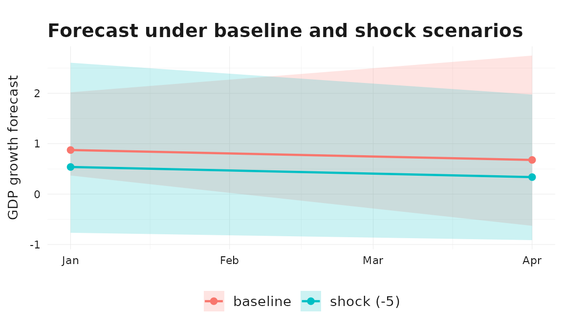
Scenario forecasts reuse the same uncertainty method and evaluate it on the supplied regressor path.

Optional Full-System Bootstrap

If you want to propagate uncertainty through the full bridge workflow, including indicator completion and aggregation, set full_system_bootstrap = TRUE. This can be substantially slower than the default residual-resampling intervals because each bootstrap draw re-estimates the full bridge pipeline. In that mode, both the reported coefficient standard errors and the forecast intervals are based on the bootstrap draws.

full_model <- mf_model(
  target = gdp_growth,
  indic = baro,
  indic_predict = "auto.arima",
  indic_aggregators = "mean",
  indic_lags = 1,
  target_lags = 1,
  h = 2,
  se = TRUE,
  full_system_bootstrap = TRUE,
  bootstrap = list(N = 20, block_length = NULL)
)

forecast(full_model)$bootstrap
#> $requested
#> [1] TRUE
#> 
#> $enabled
#> [1] TRUE
#> 
#> $N
#> [1] 20
#> 
#> $valid_N
#> [1] 20
#> 
#> $block_length
#> [1] 5

Point Forecasts Only

If you are only interested in point estimates, leave se = FALSE. In that case, bootstrap is ignored and forecast() still returns the same object shape, with NA uncertainty fields.

point_model <- mf_model(
  target = gdp_growth,
  indic = baro,
  indic_predict = "auto.arima",
  indic_aggregators = "mean",
  indic_lags = 1,
  target_lags = 1,
  h = 1,
  se = FALSE,
  bootstrap = list(N = 20)
)

forecast(point_model)
#> Mixed-frequency forecast
#> -----------------------------------
#> Target series: gdp_growth
#> Forecast horizon: 1
#> Uncertainty: point forecast only
#> -----------------------------------
#>   time       mean 
#> 1 2023-01-01 0.875

Interpretation

With the default se = TRUE, these intervals are residual-resampling prediction intervals for the fitted target equation, while coefficient standard errors come from HAC or Delta-HAC estimation. When full_system_bootstrap = TRUE, both the coefficient standard errors and the forecast intervals come from a full-system block bootstrap that resamples target-period blocks from the aligned mixed-frequency system, refits the bridge workflow on each draw, and evaluates the resulting future paths.