Ragged-Edge Nowcasting with bridgr • bridgr

Why Ragged Edges Matter

Mixed-frequency nowcasting usually happens at the ragged edge: the lower-frequency target has not been released yet, and the higher-frequency indicators are only partially observed for the current target period.

bridgr handles that situation through indic_predict, which controls how the missing high-frequency tail is completed before the target equation is estimated or forecast.

The currently supported options are:

"last": extend the latest available high-frequency observation.
"mean": extend the mean of the latest available high-frequency block.
"auto.arima": fit an automatic ARIMA model to each indicator and forecast the missing observations.
"ets": fit an ETS model to each indicator and forecast the missing observations.
"direct": do not forecast the indicator at all. Instead, align the latest observed complete high-frequency blocks directly to the target periods and average them within each target period.

A Ragged-Edge Example

We start from the package’s quarterly GDP growth series and monthly barometer, then remove the last quarterly GDP observation and the last two monthly indicator observations. That creates a clean nowcast setup: the final quarter is now forecasted rather than estimated, and the monthly indicator is only partially observed for that forecast quarter.

gdp_growth <- suppressMessages(tsbox::ts_na_omit(tsbox::ts_pc(gdp)))
gdp_nowcast <- gdp_growth |>
  dplyr::slice_head(n = nrow(gdp_growth) - 1)

baro_ragged <- baro |>
  dplyr::slice_head(n = nrow(baro) - 2)

tail(gdp_growth)
#> # A tibble: 6 × 2
#>   time       values
#>   <date>      <dbl>
#> 1 2021-07-01  2.34 
#> 2 2021-10-01  0.411
#> 3 2022-01-01  0.105
#> 4 2022-04-01  1.03 
#> 5 2022-07-01  0.255
#> 6 2022-10-01  0.102
tail(gdp_nowcast)
#> # A tibble: 6 × 2
#>   time       values
#>   <date>      <dbl>
#> 1 2021-04-01  2.47 
#> 2 2021-07-01  2.34 
#> 3 2021-10-01  0.411
#> 4 2022-01-01  0.105
#> 5 2022-04-01  1.03 
#> 6 2022-07-01  0.255
tail(baro_ragged)
#> # A tibble: 6 × 2
#>   time       values
#>   <date>      <dbl>
#> 1 2022-05-01   90.9
#> 2 2022-06-01   95.7
#> 3 2022-07-01   91.7
#> 4 2022-08-01   89.4
#> 5 2022-09-01   89.0
#> 6 2022-10-01   87.5

The target history now ends one quarter earlier, while the monthly indicator contains only a partial block for the quarter we want to nowcast.

Comparing Indicator Completion Rules

predict_methods <- c("last", "mean", "auto.arima", "ets")

models <- lapply(
  predict_methods,
  function(method) {
    mf_model(
      target = gdp_nowcast,
      indic = baro_ragged,
      indic_predict = method,
      indic_aggregators = "mean",
      target_lags = 1,
      h = 1
    )
  }
)
names(models) <- predict_methods

forecast_df <- dplyr::bind_rows(
  lapply(predict_methods, function(method) {
    fc <- forecast(models[[method]])
    dplyr::tibble(
      method = method,
      forecast_time = fc$time,
      forecast = as.numeric(fc$mean)
    )
  })
)

forecast_df
#> # A tibble: 4 × 3
#>   method     forecast_time forecast
#>   <chr>      <date>           <dbl>
#> 1 last       2022-10-01      -0.968
#> 2 mean       2022-10-01      -0.876
#> 3 auto.arima 2022-10-01      -0.706
#> 4 ets        2022-10-01      -0.968

The model specification is the same in each case. The only difference is how the missing monthly observations are completed before the indicator is aggregated to the quarterly frequency.

Visualizing the completed indicator paths

The plot below shows the tail of the observed monthly indicator together with the two extrapolated months that each indic_predict rule produces for the partially observed forecast quarter.

last_obs <- max(baro_ragged$time)
last_obs_value <- baro_ragged$values[baro_ragged$time == last_obs]
future_months <- seq(last_obs, by = "month", length.out = 3)[-1]

observed_tail <- baro_ragged |>
  dplyr::slice_tail(n = 9) |>
  dplyr::transmute(
    time = .data$time,
    value = .data$values,
    method = "observed"
  )

extended <- dplyr::bind_rows(
  lapply(predict_methods, function(method) {
    indicator_tbl <- models[[method]]$indic
    extension <- indicator_tbl |>
      dplyr::filter(.data$time %in% future_months) |>
      dplyr::transmute(
        time = .data$time,
        value = .data$values,
        method = method
      )
    # join to the last observed point for a continuous line
    dplyr::bind_rows(
      dplyr::tibble(time = last_obs, value = last_obs_value, method = method),
      extension
    )
  })
)

ggplot2::ggplot(
  dplyr::bind_rows(observed_tail, extended),
  ggplot2::aes(x = .data$time, y = .data$value, color = .data$method)
) +
  ggplot2::geom_line(linewidth = 0.8) +
  ggplot2::geom_point(size = 1.6) +
  ggplot2::labs(
    title = "Indicator completion at the ragged edge",
    x = NULL,
    y = "KOF barometer",
    color = NULL
  ) +
  theme_bridgr()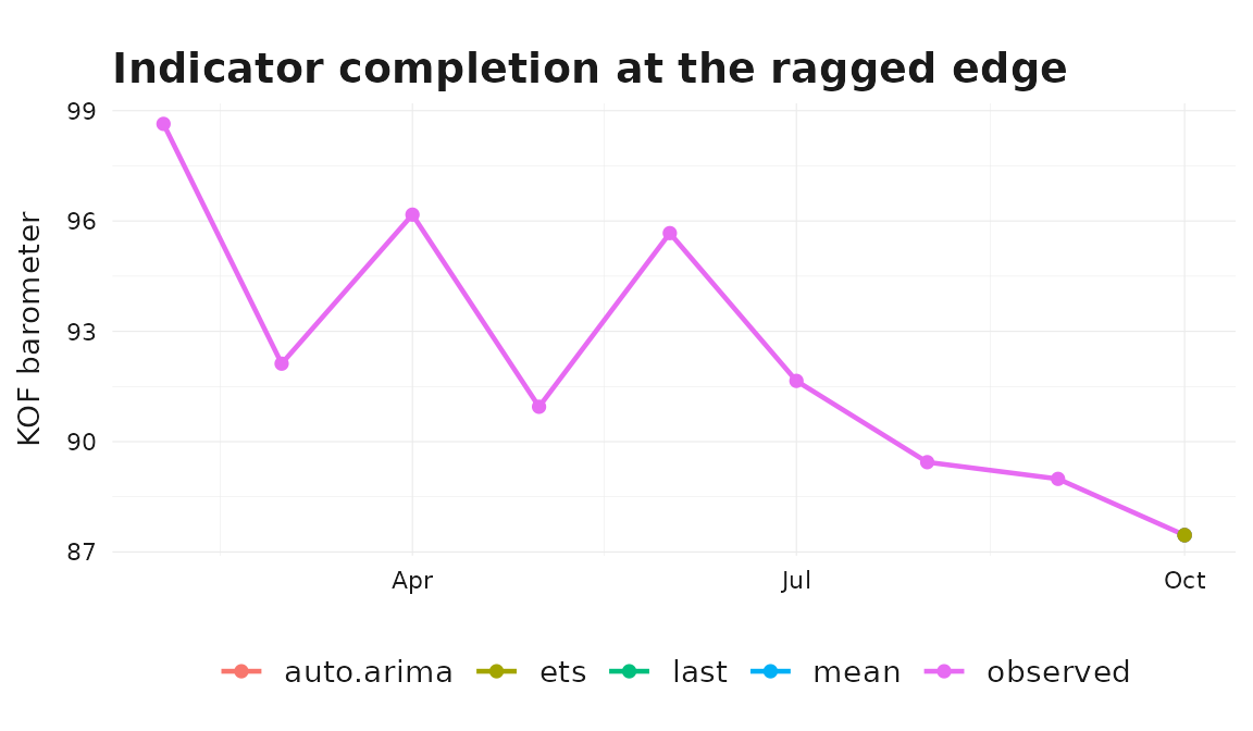

The differences across rules are exactly what their names suggest: "last" holds the last value flat, "mean" extends the mean of the recent block, and auto.arima / ets produce model-based paths.

Direct Alignment

"direct" takes a different route. The indicator is not forecasted. Instead, bridgr assigns the latest complete high-frequency blocks backward to the target periods and averages them within each target period.

direct_model <- mf_model(
  target = gdp_nowcast,
  indic = baro_ragged,
  indic_predict = "direct",
  h = 1
)

forecast(direct_model)
#> Mixed-frequency forecast
#> -----------------------------------
#> Target series: gdp_nowcast
#> Forecast horizon: 1
#> Uncertainty: point forecast only
#> -----------------------------------
#>   time       mean  
#> 1 2022-10-01 -0.150

This is especially useful when you want to avoid a separate indicator forecasting step and prefer to work only with observed high-frequency data.

Explicit Missing Values

Real-time indicator data sometimes contain explicit NA cells inside the sample, for example because of late releases or reporting holidays. Implicit ragged edges (a shorter indicator tail with no NA cells) are always supported through indic_predict. By default bridgr errors on explicit NA values; the missing argument controls what to do instead.

missing = "impute" interpolates linearly inside each series and is the most generally useful choice. The example below introduces a single internal gap and re-fits the model under both "error" (default, captured here) and "impute".

baro_internal_na <- baro_ragged
internal_gap <- seq(nrow(baro_internal_na) - 14, nrow(baro_internal_na) - 13)
baro_internal_na$values[internal_gap] <- NA_real_

invisible(tryCatch(
  mf_model(
    target = gdp_nowcast,
    indic = baro_internal_na,
    indic_predict = "last",
    indic_aggregators = "mean",
    h = 1
  ),
  error = function(e) message("Error captured: ", conditionMessage(e))
))
#> Error captured: `indic` contains missing values.

imputed_model <- mf_model(
  target = gdp_nowcast,
  indic = baro_internal_na,
  indic_predict = "last",
  indic_aggregators = "mean",
  h = 1,
  missing = "impute"
)
#> Warning in mf_model(target = gdp_nowcast, indic = baro_internal_na,
#> indic_predict = "last", : `indic` contains 2 missing values; imputing them by
#> linear interpolation within each series.

forecast(imputed_model)
#> Mixed-frequency forecast
#> -----------------------------------
#> Target series: gdp_nowcast
#> Forecast horizon: 1
#> Uncertainty: point forecast only
#> -----------------------------------
#>   time       mean  
#> 1 2022-10-01 -0.897

missing = "drop" removes NA rows entirely and is useful when those rows do not break the per-period completeness required by the inferred frequency ladder — for example when they sit beyond the estimation sample. In most ragged-edge workflows indic_predict is the better mechanism for handling trailing gaps.

When to Use Which Option

As a rough guide:

Use "last" when a simple carry-forward rule is acceptable.
Use "mean" when you want a stable deterministic fill based on the latest high-frequency block.
Use "auto.arima" or "ets" when the indicator has meaningful time-series structure and a separate extrapolation step is sensible.
Use "direct" when you want direct alignment without indicator forecasting and want to rely only on the latest observed complete high-frequency blocks.

The good part is that the downstream workflow does not change. The same summary() and forecast() interface works across all of these nowcasting choices.