MIDAS Regressions - Nowcasting US GDP growth with mixed frequency data
The recent Covid-19 crisis demonstrated how useful high-frequency data is to reflect the current state of the economy in a rapidly changing environment. However, to quantify what a change in a high-frequency variable means for a lower-frequency variable such as the growth rate of gross domestic product (GDP), methods are needed that exploit the information contained in the high-frequency indicator and link it to the low-frequency variable. A method that is able to do this is called mixed data sampling (MIDAS) regressions developed by Ghysels et. al., 2014.1 Because there are not many good online tutorials on how to apply MIDAS regressions in R, a rather flexible script for applying the method is shown here.
The objective is to predict quarterly U.S. GDP growth with the monthly variables industrial production growth and the growth rate of the number of workers in the nonfarm sector, and the weekly growth rate of continued claims, also referred to as insured unemployment. We would like to find out if the use of these variables improves the nowcasting performance compared to a simple autoregressive model of order 1 (AR(1) model). And if so, at which horizon the improvement becomes statstically significant. For this we use a pseudo realtime out-of-sample nowcasting procedure. It’s pseudo realtime because some simplifying assumptions are made. First, we assume that the variables are always published on the last day of the corresponding period (i.e. no ragged edge). In reality, macroeconomic variables are published with a substantial delay. For example, GDP is only published 1-2 months after the end of the quarter. Second, we ignore the fact that the variables are being revised over time (we only use the latest vintage).
More technically, the variable of interest is quarterly GDP growth, which is denoted as \(y_{t_q}\), where \(t_q\) is the quarterly time index \(t_q = 1,2,...,T_y\), with \(T_y\) being the last quarter for which GDP figures are available. The aim is to nowcast quarterly GDP growth, \(y_{Ty+1}\). We assume hat the information set for nowcasting includes two stationary monthly indicators \(x_{t_m}\) and one stationary weekly indicator \(x_{t_w}\) in addition to the available GDP observations. For simplicity we assume every quarter to have \(M=3\) months and \(W=12\) weeks. Hence, the time index for the monthly observations is defined as a fraction of the low-frequency quarter according to \(t_m =1-2/3,1-1/3,...,1,2-2/3,...,T_x-1/3,T_{x_m}\), where \(T_{x_m}\) is the last day for which the monthly indicator is available. Accordingly, the time index for the weekly variable is given by \(t_w =1-11/12,1-11/12,...,1,2-11/12,...,T_x-1/12,T_{x_w}\). The sample spans from January 1, 1968 to December 31, 2021. The evaluation starts in January, 1980.
The MIDAS approach is a direct multi-step forecasting tool. We use the following model
\begin{align} \label{ch1:eq.midas} y_{t_q+1} = c + \sum_{r=0}^{S-1} \alpha_r y_{t_q - r} \sum_{p=0}^{P-1} \beta_p \sum_{k=0}^{K-1} b(k, \theta)L^{(pM + k)/M} x_{t_m+T_{x_m}-T_y} + \sum_{q=0}^{P-1} \beta_q \sum_{l=0}^{L-1} b(l, \theta)L^{(qW + l)/W} x_{t_w+T_{x_w}-T_y} + \varepsilon_{t+1} \end{align}
where \(c\) is a constant, \(S\) the AR lag order, \(P\) denotes the number of low-frequency lags and \(K\) and \(L\) the number of high-frequency lags per low-frequency lag (including zero). We set \(S=1\), \(P=2\), \(K=3\) and \(L=12\), meaning the dependent variable depends on all 3 monthly and all 12 weekly values of the current and the last quarter. The lag operator is defined as \(L^{1/3}x_{t_m} = x_{t_m - 1/3}\). Because \(x_{t_w}\) is sampled at a much higher frequency than \(y_{t_q}\), we potentially have to include many high-frequency lags to achieve an adequate modelling, which easily leads to overparameterization in the unrestricted linear case. To avoid parameter proliferation, we use a non-linear weighting scheme given by the polynomials \(b(k, \theta)\) and \(b(l, \theta)\). Note that we use the same polynomial specification for all low-frequency lags included in the model.
The polynomial we use is the exponential Almon lag polynomial of order two. It has the following form
\begin{align} b(k, \theta) = \frac{exp(\theta_1 k + \theta_2 k^2)}{\sum_{j=0}^K exp(\theta_1 j + \theta_2 j^2)} \end{align}
This functional form allows for many different shapes. The weighting scheme can for instance be hump-shaped, declining or flat. By definition, they sum to one. Moreover, it parsimoniously represents the large number of predictors. The parameters are estimated by non-linear least squares (NLS).
To program the whole thing in R we start by loading the necessary packages and defining useful functions:
#------------------------------------------------------------------------------------
# Packages and functions
#------------------------------------------------------------------------------------
rm(list = ls())
library(quantmod)
library(dplyr)
library(tsbox)
library(zoo)
library(lubridate)
library(midasr)
library(ggplot2)
library(xts)
library(forecast)

# Padd NAs to x if x has not the desired length
padd_nas <- function(x, desired_length) {
  n <- length(x)
  if(n < desired_length) {
    c(rep(NA,desired_length-n),x)
  } else {
    tail(x,desired_length)
  }
}

# Get data from FRED
ts_fred <- function(..., class = "data.frame") {
  symb <- c(...)
  dta.env <- new.env()
  suppressMessages(getSymbols(symb, env = dta.env, src = "FRED"))
  z <- data.table::rbindlist(lapply(as.list(dta.env), ts_dt), idcol = "id")
  tsbox:::as_class(class)(z)
}
The next step is to define a set of parameters:
#------------------------------------------------------------------------------------
# Parameters
#------------------------------------------------------------------------------------
startDate <- as.Date("1968-01-01") # This should be the first day of a year
endDate   <- as.Date("2021-12-31") # This should be the last day of a year
startEval <- as.Date("1980-01-01") # This should be the first day of a year

AGG       <- "B"            # Estimate one lag polynomial for all lags included ("B")

noLags    <- 2              # How many lags in MIDAS model (in lf terms, including 0)
noARBench <- 1              # How many lags in benchmark AR(p) model (0 not possible)
noAR      <- 1              # How many AR lags in MIDAS model (0 possible)

lf <- 4                     # Frequency of dependent variable
mf <- 3                     # Frequency of independent mid freq variable (in terms of lf variable)
hf <- 12                    # Frequency of independent hf variable (in terms of lf variable)
lft <- "quarter"            # Low frequency label

poly <- "expalmon"          # Choose polynomial for MIDAS regresion (only expalmon ftm)

# Don't adjust below here
#--------------------------------------------------------------------------------
# Some definitions of frequencies
dpw <- 5                    # Days per week
wpm <- 4                    # Weeks per month
mpq <- 3                    # Months per quarter
dpm <- dpw*wpm              # Days per month
wpq <- wpm*mpq              # Weeks per quarter
dpq <- dpw*wpq              # Days per quarter


# Numbers per low frequency
if (lft == "quarter") {
  dplf <- dpq
  wplf <- wpq
  mplf <- mpq
} else if (lft == "month") {
  dplf <- dpm
  wplf <- wpm
  mplf <- 1
}
Then we get the data. Moreover, we adjust the series such that every quarter consists of 3 months and 12 weeks and set the dates such that every fourth week of the month has the same date as the months.
#------------------------------------------------------------------------------------
# Get the data
#------------------------------------------------------------------------------------
dtalf <- ts_fred(c("GDPC1")) %>%
  ts_pc() %>%
  ts_xts() %>%
  ts_span(start=startDate)

dtamt <- ts_fred(c("INDPRO", "PAYEMS")) %>%
  ts_pc() %>%
  ts_wide() %>%
  mutate(time = round_date(time, unit="day"),
         year = year(time),
         quarter = quarter(time)) %>%
  group_by(year, quarter) %>% # make sure every quarter consists of 3 months
  arrange(time) %>%
  slice((n()-2):n()) %>%
  mutate(period = row_number()) %>%
  ungroup() %>%
  mutate(time = ceiling_date(time, unit = "month") %>% rollback())

dtawk <- ts_fred(c("ICSA", "CCSA")) %>%
  ts_pc() %>%
  ts_wide() %>%
  ts_span(end="2022-03-31") %>%
  mutate(time = round_date(time, unit="day"),
         year = year(time),
         quarter = quarter(time),
         month =  month(time)) %>%
  group_by(year, month) %>% # make sure every month consists of 4 weeks
  arrange(time) %>%
  slice((n()-3):n()) %>% # if a month has 5 weeks drop first week of month
  mutate(periodM = row_number()) %>%
  ungroup() %>%
  group_by(year, quarter) %>% # make sure every quarter consists of 12 weeks
  arrange(time) %>%
  slice((n()-11):n()) %>% # if a month has 13 weeks drop first week of month
  mutate(period = row_number()) %>%
  ungroup()  %>%
  mutate(time = ceiling_date(time, unit = "week") -1 ,
         time = if_else(period %in% c(4,8,12) & time != (ceiling_date(time, "month") - 1), rollforward(time), time))


periodNumbersWeek <- dtawk %>%
  select(time, period)

periodNumbersMonth <- dtamt %>%
  select(time, period)


vintVar   <- dtalf
depVarLab <- "GDP"

IndMFLab    <- c("INDPRO", "PAYEMS")
IndMF       <- dtamt %>% # Mid frequency indicator
  select(time, all_of(IndMFLab)) %>%
  ts_long() %>%
  ts_xts()


IndHFLab    <- c("CCSA")
IndHF       <- dtawk %>% # High frequency indicator
  select(time, all_of(IndHFLab)) %>%
  ts_long() %>%
  ts_xts()

# Initialize empty arrays for nowcasts
FcstMidas.h0 <- xts::xts(matrix(NA, nrow=nrow(vintVar), ncol = (hf+11)), order.by = zoo::index(vintVar))
colnames(FcstMidas.h0) <- paste0("hor",0:(hf+10))
FcstMidas.h0[,] <- NA
FcstMidas.IT.h0 <- FcstMidas.h0
FcstAR.h0 <- FcstMidas.h0
FcstMean.h0 <- FcstMidas.h0

# Final value for computing forecast errors
Y.final <- (vintVar[,ncol(vintVar)])
Then we estimate the model and calculate a nowcast within a for loop.
#------------------------------------------------------------------------------------
# Estimate Models
#------------------------------------------------------------------------------------
DataPlot <- NULL
firstRound <- TRUE
oldPeriod <- floor_date(zoo::index(IndHF)[1], lft)
for (currDate in as.character(zoo::index(IndHF))) {
  message(currDate)
  currDate <- as.Date(currDate)
  newPeriod <- floor_date(currDate, lft)

  # At beginning of new lf period, reset dates
  if(newPeriod > oldPeriod) {
    Date.h0 <- floor_date(currDate, lft)
    Date.h1 <- add_with_rollback(Date.h0, months(mplf), roll_to_first = T)

    # Number of intraperiod forecasts
    hfh <- nrow(ts_span(IndHF, start=Date.h0, end=Date.h1 %>% rollback() ))
    hfh.max <- hfh

    if(currDate >= startEval) {
      # Construct dependent data
      Y.h0    <- vintVar %>% ts_span(start = startDate, end = Date.h0)
      Y.h0[nrow(Y.h0)][1,] <- NA
    }
  }

  if(currDate < startEval ) {
    oldPeriod <- newPeriod
    next
  }
  if(currDate > endDate) {break}

  # Construct independent data for MIDAS mid frequency
  xM <- matrix(NA, nrow = length(Y.h0), ncol = mf*noLags)
  if (!currDate %in%  periodNumbersMonth$time) {
    currentPeriod <- periodNumbersMonth[periodNumbersMonth$time==floor_date(currDate, "month") -1,]$period
  } else {
    currentPeriod <- periodNumbersMonth[periodNumbersMonth$time==currDate,]$period
  }

  periodIndex <- currentPeriod + 1

  startTime <- startDate
  if (noLags > 1) {
    for (lag in 1:(noLags)) {startTime <- floor_date(rollback(startTime), lft)}
  }
  for (var in 1:ncol(IndMF)) {
    tmp <- ts_span(IndMF,start = startTime)[,var]
    for(lag in 1:(length(Y.h0))) {
      xM[lag,] <- head(rev(padd_nas(tmp[(mf*(lag-1) + periodIndex):(mf*(lag-1) + periodIndex + noLags*mf-1)], noLags*mf)),noLags*mf)
    }
    assign(paste0("xM.",var), xM)
  }

  # Construct independent data for MIDAS high frequency
  xW <- matrix(NA, nrow = length(Y.h0), ncol = hf*noLags)
  currentPeriod <- periodNumbersWeek[periodNumbersWeek$time==currDate,]$period

  periodIndex <- currentPeriod + 1

  startTime <- startDate
  if (noLags > 1) {
    for (lag in 1:(noLags)) {startTime <- floor_date(rollback(startTime), lft)}
  }
  for (var in 1:ncol(IndHF)) {
    tmp <- ts_span(IndHF,start = startTime)[,var]
    for(lag in 1:(length(Y.h0))) {
      xW[lag,] <- head(rev(padd_nas(tmp[(hf*(lag-1) + periodIndex):(hf*(lag-1) + periodIndex + noLags*hf-1)], noLags*hf)),noLags*hf)
    }
    assign(paste0("xW.",var), xW)
  }

  # Estimation
  # Midas
  if(noAR > 0){
    if (noAR == 1) {
      formula <- paste0("Y.h0 ~  mls(Y.h0, 1, 1) ")
    } else {
      formula <- paste0("Y.h0 ~  mls(Y.h0, 1:",noAR,", 1) ")
    }
  } else {
    formula <- paste0("Y.h0 ~ ")
  }
    startvals <- list()
    for (var in 1:ncol(IndMF)) {
      assign(paste0("xm.",var), as.numeric(t(get(paste0("xM.",var))[,mf:1])))
      formula <- paste0(formula, "+ mls(xm.",var,", 0:(mf*noLags-1), mf, amweights, nealmon, AGG)")
      startvals[[paste0("xm.",var)]] <- c(rep(-0.1,noLags), 0.0005, 0.0005)
    }

    for (var in 1:ncol(IndHF)) {
      assign(paste0("xw.",var), as.numeric(t(get(paste0("xW.",var))[,hf:1])))
      formula <- paste0(formula, "+ mls(xw.",var,", 0:(hf*noLags-1), hf, amweights, nealmon, AGG)")
      startvals[[paste0("xw.",var)]] <- c(rep(-0.1,noLags), 0.0005, 0.0005)
    }

    while (TRUE) { # loop because initial starting values might not converge
      Y.h0 <- as.numeric(Y.h0)
      formula <- as.formula(formula)
      Model.Midas.h0 <-  tryCatch({midasr::midas_r(formula,
                                                   start=startvals)},
                                  error=function(e){return("try-error")})
      if (class(Model.Midas.h0) != "midas_r") {
        startval <- rnorm(length(c(rep(-0.1,noLags), 0,0)),0,00.1)+c(rep(-0.1,noLags), 0,0)
        for (var in 1:ncol(IndMF)) {
          startvals[[paste0("xm.",var)]] <- startval
        }
        for (var in 1:ncol(IndHF)) {
          startvals[[paste0("xw.",var)]] <- startval
        }
      } else {
        break
      }
    }

    coef.h0 <- coef(Model.Midas.h0, midas = T)

  # AR
  Model.AR <- Arima(Y.h0[!is.na(Y.h0)], order = c(noARBench, 0, 0), include.constant= TRUE)

  # Construct independent predictors for MIDAS
  for (var in 1:ncol(IndMF)) {
    newx <- c(ts_span(IndMF[,var], end = currDate)) %>% as.numeric()
    newx <- head(rev(newx),(mf*noLags))
    assign(paste0("midasXM",var), matrix(newx,nrow=1, ncol=mf*noLags, byrow=T))
  }

  for (var in 1:ncol(IndHF)) {
    newx <- c(ts_span(IndHF[,var], end = currDate)) %>% as.numeric()
    newx <- head(rev(newx),(hf*noLags))
    assign(paste0("midasXW",var), matrix(newx,nrow=1, ncol=hf*noLags, byrow=T))
  }

  # Forecasting
  # Midas
  midasX <- 1
  for (var in 1:ncol(IndMF)) {
    midasX <- c(midasX, get(paste0("midasXM", var)))
  }
  for (var in 1:ncol(IndHF)) {
    midasX <- c(midasX, get(paste0("midasXW", var)))
  }

  arMIDAS <- Y.h0[!is.na(Y.h0)][(length(Y.h0[!is.na(Y.h0)])+1-noAR):length(Y.h0[!is.na(Y.h0)])]

  Fcst.Midas.h0 <- coef.h0[!grepl("Y.h0", names(coef.h0))]%*%midasX + coef.h0[grepl("Y.h0", names(coef.h0))]%*%rev(arMIDAS) %>% as.numeric()

  FcstMidas.h0[Date.h0, hfh] <- Fcst.Midas.h0


  # AR
  Fcst.AR     <- forecast(Model.AR, h = 2, level = c(50, 80, 90, 95))
  Fcst.AR.h0 <- Fcst.AR$mean[1]

  FcstAR.h0[Date.h0, hfh] <- Fcst.AR.h0

  DataPlot <- bind_rows(DataPlot,
                        tibble(value = Fcst.Midas.h0,
                               time = Date.h0,
                               currDate = currDate,
                               horizon = hfh,
                               id = "h0",
                               model = "midas"),
                        tibble(value = Fcst.AR.h0,
                               time = Date.h0,
                               currDate = currDate,
                               horizon = hfh,
                               id = "h0",
                               model = "ar")
  )

  oldPeriod <- newPeriod
  hfh <- hfh - 1
}
Finally, we calculate the nowcasting errors, conduct Diebold-Mariano-West (DMW) tests and plot the results.
#------------------------------------------------------------------------------------
# Plot Results
#------------------------------------------------------------------------------------

# Calculate errors
ErrMidas.h0 <- sweep(as.matrix(FcstMidas.h0), 1, as.matrix(Y.final))[,1:(hf)]
ErrAR.h0 <- sweep(as.matrix(FcstAR.h0), 1, as.matrix(Y.final))[,1:(hf)]

# RMSE all data
RMSEMIDAS.h0 <- apply(ErrMidas.h0,2, function(x){sqrt(mean(x^2, na.rm=T))})
RMSEAR.h0 <- apply(ErrAR.h0,2, function(x){sqrt(mean(x^2, na.rm=T))})

# RMSE excluding covid
exCovid.h0 <-  !rownames(ErrMidas.h0) %in% c("2020-01-01","2020-04-01","2020-07-01", "2020-10-01")
RMSEMIDAS.exC.h0 <- apply(ErrMidas.h0[exCovid.h0,],2, function(x){sqrt(mean(x^2, na.rm=T))})
RMSEAR.exC.h0 <- apply(ErrAR.h0[exCovid.h0,],2, function(x){sqrt(mean(x^2, na.rm=T))})

# Plot all
p <- bind_rows(tibble(RMSE = RMSEMIDAS.h0,
                      horizon = 0:(hf-1),
                      id = "H0",
                      model = "MIDAS"),
               tibble(RMSE = RMSEAR.h0,
                      horizon = 0:(hf-1),
                      id = "H0",
                      model = "AR")
) %>%
  ggplot(aes(x=horizon, y=RMSE, colour=model)) +
  geom_line() +
  scale_x_reverse() +
  scale_color_brewer(palette="Set1") +
  theme_bw() +
  theme(title = element_blank())
#p
#ggsave(paste0("RMSE_H0_FS_",poly,"_",AGG,"_CC.pdf"))

# Plot exclding covid
p<-bind_rows(tibble(RMSE = RMSEMIDAS.exC.h0,
                    horizon = 0:(hf-1),
                    id = "H0",
                    model = "MIDAS"),
             tibble(RMSE = RMSEAR.exC.h0,
                    horizon = 0:(hf-1),
                    id = "H0",
                    model = "AR")
) %>%
  ggplot(aes(x=horizon, y=RMSE, colour=model)) +
  geom_line() +
  scale_x_reverse() +
  scale_color_brewer(palette="Set1") +
  theme_bw() +
  theme(title = element_blank())
p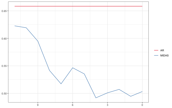
#ggsave(paste0("RMSE_H0_exCovid_",poly,"_",AGG,"_CC.pdf"))

# Plot actual vs nowcast (horizon 0)
p <- DataPlot %>%
  filter(horizon==1) %>%
  #filter(time >= "2007-01-01" & time < "2010-01-01") %>%
  filter(model == "midas") %>%
  ggplot() +
  geom_line(aes(x=time, y=value, colour="nowcast")) +
  geom_line(data = ts_tbl(Y.final) %>%
              ts_span(start=startEval,
                      end= "2021-12-31"
              ),
            aes(x=time, y=value, colour="GDP growth")) +
  #scale_y_continuous(limits = c(-2.8,2)) +
  theme_bw() +
  theme(title = element_blank())
p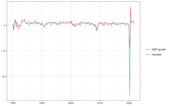
#ggsave(paste0("RealTimeForecastMIDAS_",poly,"_",AGG,"_CC.pdf"))

# DMW tests incl. plot
ref.h0 <- ErrAR.h0
models.h0 <- list(ErrMidas.h0)
modelNames <- c("Midas")

index.h0 <- 1:nrow(ErrMidas.h0)
index.h0 <- exCovid.h0

dta <- tibble()
for (h in c(1:12)) {
  for (model in 1) {
    Err.h0 <- na.omit(models.h0[[model]][index.h0,h])
    ErrRef.h0 <- na.omit(na.omit(ref.h0[index.h0,h]))
    Test.h0 <- dm.test(Err.h0, ErrRef.h0, alternative = c("less"), h = 1, power = 2)

    dta <- bind_rows(dta, tibble(h=h-1,
                                 Model=modelNames[model],
                                 `relative RMSE` = sqrt(mean(Err.h0^2, na.rm=T))/sqrt(mean(ErrRef.h0^2, na.rm=T)),
                                 `DMW (p-value)` = Test.h0$p.value
    )
    )
  }
}

dta <- dta %>%
  arrange(h)

p <- filter(dta, Model == "Midas") %>%
  mutate(pval = factor(if_else(`DMW (p-value)` > 0.1, "> 0.1",
                               if_else(`DMW (p-value)` <= 0.1 & `DMW (p-value)` > 0.05, "< 0.1",
                                       if_else(`DMW (p-value)` <= 0.05 & `DMW (p-value)` > 0.01, "< 0.05",
                                               if_else(`DMW (p-value)` <= 0.01, "< 0.01", "Not")))),
                       levels = c("> 0.1", "< 0.1", "< 0.05", "< 0.01"))) %>%
  ggplot() +
  geom_line(aes(x=h, y=`relative RMSE`)) +
  geom_point(aes(x=h, y=`relative RMSE`, color=(pval))) +
  scale_x_reverse() +
  scale_color_brewer(palette="Set2") +
  #scale_color_gradient2(midpoint=0.2, low="green", mid="yellow",
  #                     high="red" ) +
  theme_bw() +
  xlab("Horizon (weeks)") +
  ylab("rel. RMSE") +
  theme(legend.title = element_blank())

p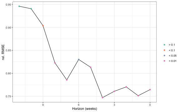
#ggsave(paste0("DMW_exCovid_Midas_AR_",poly,"_",AGG,"_CC",".pdf"))The results show that the used high-frequency variables indeed provide valuable information about current quarter GDP growth. The MIDAS nowcast outperfroms statistically significantly the AR(1) model after about 2 weeks of the current quarter.
-
Ghysels E, Santa-Clara P, Valkanov R (2002). “The MIDAS Touch: Mixed Data Sampling Regression Models.” Working paper, UNC and UCLA. ↩
Comments You need to have a GitHub Account to comment!
Post comment