Predicting the default of lending club loans

[ #machine-learning #R ]

This is based on a project I conducted in a GSERM course in “Advanced Machine Learning with R”. I develop a ML model to predict the default of lending club loans. We got training data and some observations with unknown outcome which was to be predicted. The predictions I got with the procedure below had an AUC of 0.7304, which was one of the highest ever achieved in this class.

Note: Calculations of the models are quite time consuming.

Let’s start loading the required packages and define some functions

library(pROC)
library(caret)
library(dplyr)
library(stringr)
library(funModeling)
library(tm)
library(topicmodels)
library(tidytext)
set.seed(123)

# Creaty dummy variable fos missing/non missing
binary_na <- function(x) {
  return (if_else(is.na(x), 1, 0))
}

# helper function for the plots
tuneplot <- function(x) {
  ggplot(x) +
    coord_cartesian(ylim = c(min(x$results$ROC), max(x$results$ROC))) +
    theme_bw()
}

Load Data

Then I load the training and test data. Further the training data is again split into 50% training set and 25% / 25% validation set to validate single models and the stack model. Then we combine those datasets again for the feature engineering.

lc <- read.csv("lending_club_train.csv", stringsAsFactors = FALSE)

# load the test dataset
lc_test <- read.csv("lending_club_test.csv", stringsAsFactors = FALSE)

trainIndex <- createDataPartition(lc$id, p = .5, 
                                  list = FALSE, 
                                  times = 1)

lc_train <- lc[trainIndex,]
lc_val <- lc[-trainIndex,]

valIndex <- createDataPartition(lc_val$id, p = .5, 
                                  list = FALSE, 
                                  times = 1)

lc_val1 <- lc_val[valIndex,]
lc_val2 <- lc_val[-valIndex,]

lc <- bind_rows(lc_train %>% mutate(data_source = "train"),
            lc_val1 %>% mutate(data_source = "validate1"),
            lc_val2 %>% mutate(data_source = "validate2"),
            lc_test %>% mutate(data_source = "test", default = NA_integer_)
          )

Feature Engineering

External Data

On top on the data provided by lending club I also use the unemploymentrate in 2016 per state and the interest rate (FEDFUNDS) in the year of the earliest cr line. It turns out, those features are not really relevant.

# load external data unemploymentrate
load("unemp.RData")
unemp <- df
colnames(unemp) <- c("names","unemp","rank","addr_state")
unemp <- unemp %>% 
  mutate(rank = as.numeric(rank),
         unemp = as.numeric(unemp))

# load external data interest rate
int_rate <- read.csv("FEDFUNDS.csv", stringsAsFactors = F) %>%
  mutate(DATE = as.numeric(substring(DATE, 0, 4)),
         FEDFUNDS = as.numeric(FEDFUNDS)) %>%
  add_row(DATE=seq(1944,1954,1), FEDFUNDS=rep(2,11))
colnames(int_rate) <- c("earliest_cr_line", "int_rate") 

# Have a look at missings uniques zeros etc.
lc_meta <- funModeling::df_status(lc, print_results = FALSE)

Topic Modelling

To get information out of the employment title I use a topic modelling algorithm with k=80 topics (or job categories). For that purpose I use an LDA (Latent Dirichlet Allocation) algorithm. In short, words that appear often together are asigned to the same topic. First of all the text is cleaned (punctuation numbers and stopwords removed) and then feed into the algorithm. The topic feature is among the 20 best features in the xgbm algorithm, thus improving the predictions by a substantial degree. The code is in the chunck below:

# Clean the emp_title
tm <- lc %>%
  select(id,emp_title) %>%
  mutate(emp_title = tolower(emp_title)) %>%
  mutate(emp_title = gsub("[[:punct:]]", " ", emp_title)) %>%
  mutate(emp_title = gsub("\\d", " ", emp_title)) %>%
  mutate(emp_title = gsub("^\\s*$", "missing", emp_title))  %>%
  unnest_tokens(word, emp_title) %>%
  anti_join(stop_words) %>%
  filter(nchar(word) > 2) %>%
  count(id, word, sort = TRUE)

# create document-term-matrix  
dtm <- tm %>% cast_dtm(id, word, n)

# run lda algorithm
lda <- LDA(dtm, k = 80, control = list(seed = 1234))

# extract relevant information
lda_gamma <- tidy(lda, matrix = "gamma")
lda_beta <- tidy(lda, matrix = "beta")

# remove again to save memory
rm(list="lda")
gc()

# Find top terms per topic
top_terms <-lda_beta %>%
  group_by(topic) %>%
  top_n(5, beta) %>%
  ungroup() %>%
  arrange(topic, -beta)

# here some helper dataframes
pd <- lda_gamma %>%
  group_by(document) %>%
  top_n(1, gamma) %>%
  ungroup() %>% 
  rename(id = document) %>%
  mutate(id = as.integer(id))

pd_nd <- pd[!duplicated(pd$id),]

fake_join <- tibble(id=seq(1,650000,1), topic = NA)

pdj <- full_join(fake_join,pd_nd, by="id") %>%
  select(c("id", "topic.y")) %>%
  rename(topic = topic.y) %>%
  mutate(topic = ifelse(is.na(topic),4,topic))

Feature Engineering

Here I do the actual engingeering, that is I convert to numeric and to factor, impute missing values and I create some possibly useful features out of the existing features.

# Select numeric features with less than 25% misssing values and impute median
lc2_nna <- lc %>%
  select(c(filter(lc_meta, p_na <25)$variable)) %>%
  select_if(is.numeric) %>% 
  mutate_all(~ifelse(is.na(.),median(., na.rm = T), .)) %>%
  # use log for annual inc
  mutate(annual_inc = log(annual_inc)) %>%
  mutate_all(~ifelse(is.infinite(.),0, .)) %>%
  select(-c("id", "default"))

# Select feature with more than 25% missings
lc2_na <- lc %>%
  select(c(filter(lc_meta, p_na > 25)$variable))

# create mvp for features containing joint in name
joint <- lc %>%
  select(contains("joint")) %>%
  mutate(verification_status_joint = ifelse(verification_status_joint=="",NA,verification_status_joint)) %>%
   mutate(joint_mvp = paste0(binary_na(.[[1]]),
                           binary_na(.[[2]]),
                           binary_na(.[[3]]),
                           binary_na(.[[4]]))) %>%
   select(joint_mvp)

# create mvp for features starting with mnth
mnth <- lc2_na %>%
  select(starts_with("mths")) %>% 
  mutate(bna1 = binary_na(.[[1]]),
         bna2 = binary_na(.[[2]]),
         bna3 = binary_na(.[[3]]),
         bna4 = binary_na(.[[4]]),
         bna5 = binary_na(.[[5]]),
         bna6 = binary_na(.[[6]]) ) %>%
  mutate_all(~ifelse(is.na(.),1200, .)) 

# create mvp for features starting with tot
tot <- lc2_na %>%
  select(starts_with("tot")) %>%
  mutate(tot_mvp = paste0(binary_na(.[[1]]),
                           binary_na(.[[2]])
                           )) %>%
  select(tot_mvp)

# create mvp for features starting with open
open <- lc2_na %>%
  select(starts_with("open")) %>%
  mutate(open_mvp = paste0(binary_na(.[[1]]),
                           binary_na(.[[2]]),
                           binary_na(.[[3]]),
                           binary_na(.[[4]]),
                           binary_na(.[[5]]),
                           binary_na(.[[6]])
                           )) %>%
  select(open_mvp)

# Feature Engineering
lc1 <- lc %>% 
  # select variables to to feature engineering
  select( default, loan_amnt, term, emp_title, emp_length, home_ownership, annual_inc, purpose, earliest_cr_line,
          revol_util, desc, addr_state, zip_code, initial_list_status, data_source, id, application_type) %>% 
  # convert to factor
  mutate(term = factor(term)) %>% 
  # is manager or equivalent?
  mutate(manager = ifelse(grepl("manager|manajer|management|president|director|senior",emp_title, ignore.case = T),1,0)) %>% 
  # is junior or equivalent?
  mutate(assist = ifelse(grepl("junior|assista",emp_title, ignore.case = T),1,0)) %>% 
  # is nurse?
  mutate(nurse = ifelse(grepl("nurse",emp_title, ignore.case = T),1,0)) %>% 
  # works in sales?
  mutate(sales = ifelse(grepl("sales",emp_title, ignore.case = T),1,0)) %>% 
  # works in service?
  mutate(service = ifelse(grepl("service",emp_title, ignore.case = T),1,0)) %>% 
  # mutate employment to favtor with less levels
  mutate(employment = ifelse(grepl("n/a",emp_length), "unemployed", emp_length)) %>% 
  mutate(employment = ifelse(grepl("< 1 year|1 year", employment), "less than 2 years", employment)) %>% 
  mutate(employment = ifelse(grepl("2 years|3 years|4 years", employment), "2-4 years", employment)) %>% 
  mutate(employment = ifelse(grepl("5 years|6 years|7 years|8 years|9 years",employment), "5-9 years", employment)) %>%       mutate(employment = factor(employment)) %>% 
  # mutate ownership to favtor with less levels
  mutate(home_ownership = ifelse(grepl("MORTGAGE|OWN", home_ownership), 1,0)) %>% 
  # higher loan than income?
  mutate(higherLTI = ifelse(loan_amnt>annual_inc,1,0)) %>% 
  # as factor
  mutate(purpose = factor(purpose)) %>% 
  # to numeric
  mutate(revol_util = as.numeric(gsub("%","",revol_util))) %>% 
  # impute mean
  mutate(revol_util =  ifelse(is.na(revol_util),mean(revol_util,na.rm = T), revol_util)) %>% 
  # use loan description ength
  mutate(desc = str_length(desc))  %>%
  # as factor
  mutate(addr_state = factor(addr_state)) %>% 
  # as factor
  mutate(application_type = factor(application_type)) %>% 
  # remove duplicated
  select(-c(emp_length, emp_title, loan_amnt, annual_inc)) %>% 
  # to numeric
  mutate(earliest_cr_line = as.numeric(gsub("\\D", "", earliest_cr_line))) %>%
  # to numeric
  mutate(zip_code = as.numeric(substr(zip_code, 0, 3))) %>%
  # as factor
  mutate(initial_list_status = factor(initial_list_status))

# bind all features to one dataframe
lc3 <- bind_cols(lc1,lc2_nna, tot, open, mnth, joint) %>% 
  select(-c(fico_range_low)) %>% 
  inner_join(unemp,by="addr_state") %>% 
  inner_join(int_rate,by="earliest_cr_line") %>% 
  inner_join(pdj,by="id") %>% 
  select(-c("names")) %>%
  mutate(addr_state = as.factor(addr_state),
         tot_mvp = as.factor(tot_mvp),
         open_mvp = as.factor(open_mvp),
         joint_mvp = as.factor(joint_mvp),
        earliest_cr_line = as.factor(earliest_cr_line))

# split to train again
lc4_train <- lc3 %>% filter(data_source == "train") %>% 
  select(-c(data_source, id)) %>%
  mutate(default = factor(default, levels = c(0, 1), labels = c("no", "yes")))

# Create Test Dataset 1
lc4_test <- lc3 %>% filter(data_source == "validate1") %>% 
  select(-c(data_source, id)) %>%
  mutate(default = factor(default, levels = c(0, 1), labels = c("no", "yes")))

# Create Test Dataset 2
lc4_test2 <- lc3 %>% filter(data_source == "validate2") %>% 
  select(-c(data_source, id)) %>%
  mutate(default = factor(default, levels = c(0, 1), labels = c("no", "yes")))

# save for faster use later
save(lc3, lc4_train, lc4_test, lc4_test2, top_terms, file="ttdata.RData")

# Remove unnecessary data to save memory
rm(list = ls())
gc()

Explore Data

Let’s do some plots to explore wether some features have predictive power to predict defaults. The following are the main findings:

Different topics have indeed different default probabilities. E.g. topic 52 has a high probability. This topic is assiciated with words like worker, warehouse and physical. This topic could therefore be related to physical labor in the warehouse.
We see more defaults when the term is 60 months rather than 36 months.
It seems also that people in Nevada tend to default.
Finally the higher debt to income ratio and or higher the loan amaunt, the higher the default probability.

# Load the data from feature engineering
load("ttdata.RData")

# Create Test Set for final predictions
#lc4_test_final <- lc3 %>% filter(data_source == "test")

# Create full Training dataset
train <- lc3 %>% filter(data_source ==  "train" | data_source == "validate1" | data_source == "validate2")  %>%
  select(-c(data_source, id)) %>%
  mutate(default = factor(default, levels = c(0, 1), labels = c("no", "yes")))

# Default by Topic
prop <- as.data.frame(table(select(train, c("default", "topic"))))
p <- ggplot(prop, aes(x=topic, y=Freq, fill = as.factor(default))) +
 geom_bar(position="fill", stat="identity") +
  theme_bw()
p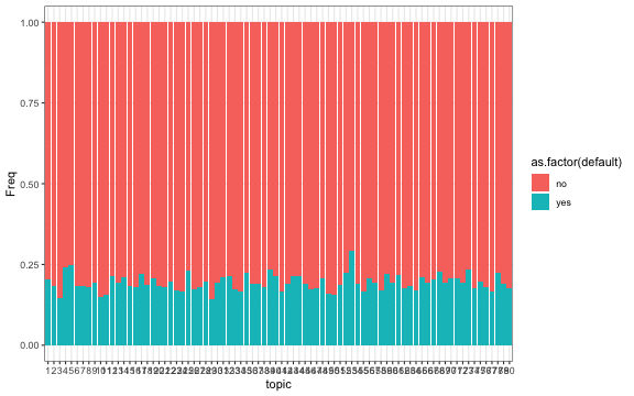

plot of chunk Explore Data

# List top 5 terms of Topic 52
top_terms %>% 
  filter(topic == 52) %>%
  select(term) %>%
  head()

## # A tibble: 5 × 1
##   term        
##   <chr>       
## 1 worker      
## 2 warehouse   
## 3 social      
## 4 professional
## 5 physical

# Default by Term
prop <- as.data.frame(table(select(train, c("default", "term"))))
p <- ggplot(prop, aes(x=term, y=Freq, fill = as.factor(default))) +
 geom_bar(position="fill", stat="identity") +
  theme_bw()
p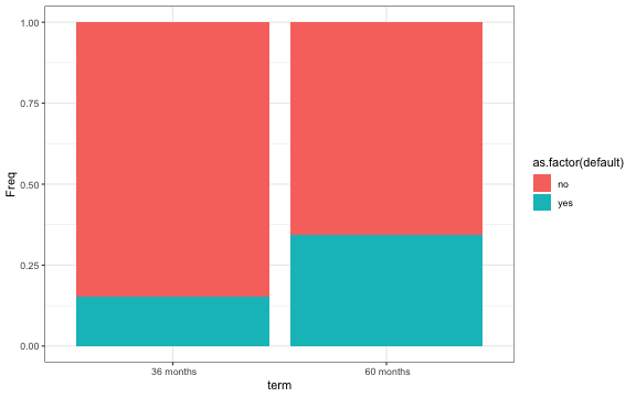

plot of chunk Explore Data

# Default by State
prop <- as.data.frame(table(select(train, c("default", "addr_state"))))
p <- ggplot(prop, aes(x=addr_state, y=Freq, fill = as.factor(default))) +
 geom_bar(position="fill", stat="identity") +
  theme_bw()
# NE and MI pretty high
p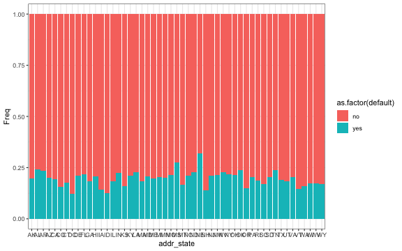

plot of chunk Explore Data

# Default by  loan amount
p <- ggplot(train, aes(x=loan_amnt , fill = as.factor(default))) +
  geom_density(adjust=2,
               alpha=0.5) +
  theme_bw()
p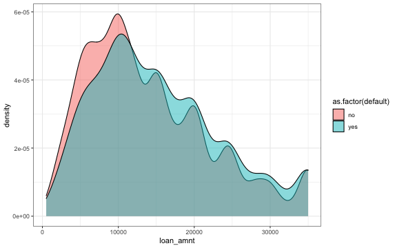

plot of chunk Explore Data

# Default by DTI
p <- ggplot(train, aes(x=dti , fill = as.factor(default))) +
  geom_density(adjust=2,
               alpha=0.5) +
  scale_x_continuous(limits=c(0,50)) +
  theme_bw()
p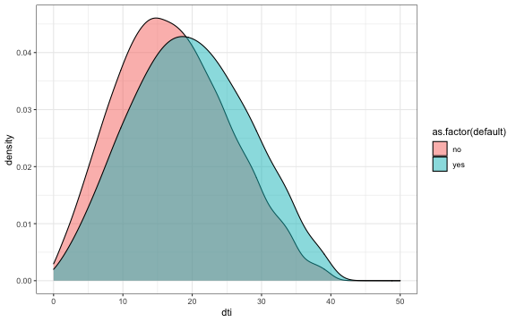

plot of chunk Explore Data

Modeling

Turning to the interesting point. In total I use 6 different models to predict defaults. Afterwards those models are evaluated with respect to the AUC. First of all, I set up the models using 3-fold cross-validation and start with a grid search to find the optimal parameter values. I use the following models:

c50
Rpart
logistic regression
elastic net regression
ranger (Random Forest)
Extreme Gradient Boosting

ctrl <- trainControl( # create a caret trainControl object
  method = "cv",
  number = 3, # 3-fold CV
  selectionFunction = "best", # select the best performer
  classProbs = TRUE, # requested the predicted probs (for ROC)
  summaryFunction = twoClassSummary, # needed to produce the ROC/AUC measures
  savePredictions = TRUE, # needed to plot the ROC curves
  allowParallel = TRUE
)

grid <- expand.grid(winnow = FALSE, trials=c(1,2,3), model="tree" )

m.c50 <- train(default ~., 
               data = lc4_train,
               method = "C5.0",
               trControl = ctrl,
               tuneGrid = grid,
               metric = "ROC")

save(m.c50, file = "m.c50.RData")

lc4_test$pred.c50 <- predict(m.c50, lc4_test, type ='prob')$yes
lc4_test2$pred.c50 <- predict(m.c50, lc4_test2, type ='prob')$yes

load("m.c50.RData")

tuneplot(m.c50)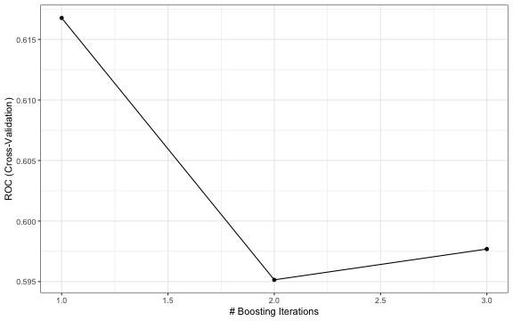

plot of chunk c50 plots

m.c50.bestTune <- m.c50$bestTune
save(m.c50.bestTune, file="m.c50.best.RData")

# Free Memory
rm(m.c50)
gc()

##             used   (Mb) gc trigger   (Mb) limit (Mb)   max used   (Mb)
## Ncells   4914970  262.5   61282001 3272.9         NA   57406743 3065.9
## Vcells 390997375 2983.1 1056106321 8057.5      16384 1276798865 9741.3

ctrl <- trainControl( # create a caret trainControl object
  method = "cv",
  number = 3, # 3-fold CV
  selectionFunction = "best", # select the best performer
  classProbs = TRUE, # requested the predicted probs (for ROC)
  summaryFunction = twoClassSummary, # needed to produce the ROC/AUC measures
  savePredictions = TRUE, # needed to plot the ROC curves
  allowParallel = TRUE
)

m.rpart <- train(default ~., 
               data = lc4_train,
               method = "rpart",
               trControl = ctrl,
               tuneLength = 10,
               metric = "ROC")

save(m.rpart, file="m.rpart.RData")

lc4_test$pred.rpart <- predict(m.rpart, lc4_test, type ='prob')$yes
lc4_test2$pred.rpart <- predict(m.rpart, lc4_test2, type ='prob')$yes

load("m.rpart.RData")

tuneplot(m.rpart)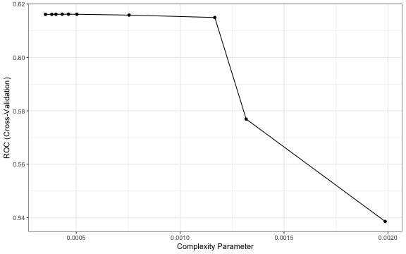

plot of chunk rpart plots

m.rpart.bestTune <- m.rpart$bestTune
save(m.rpart.bestTune, file="m.rpart.best.RData")

# Free Memory
rm(m.rpart)
gc()

##              used   (Mb) gc trigger    (Mb) limit (Mb)   max used   (Mb)
## Ncells    4959808  264.9   39220481  2094.6         NA   57406743 3065.9
## Vcells 1140240105 8699.4 1526733908 11648.1      16384 1276798865 9741.3

tune_control <- caret::trainControl(
  method = "cv", # cross-validation
  number = 3, # with n folds 
  verboseIter = FALSE, # no training log
  classProbs = TRUE, # requested the predicted probs (for ROC)
  summaryFunction = twoClassSummary, # needed to produce the ROC/AUC measures
  selectionFunction = "best",
  savePredictions = TRUE, # needed to plot the ROC curves
  allowParallel = TRUE # FALSE for reproducible results 
)

m.glm <- caret::train(
  form = default ~., 
  data = lc4_train,
  trControl = tune_control,
  method = "glm",
  family = "binomial",
  metric = "ROC"
)

save(m.glm, file="m.glm.RData")

lc4_test$pred.glm <- predict(m.glm, lc4_test, type ='prob')$yes
lc4_test2$pred.glm <- predict(m.glm, lc4_test2, type ='prob')$yes

tune_control <- caret::trainControl(
  method = "cv", # cross-validation
  number = 3, # with n folds 
  #index = createFolds(tr_treated$Id_clean), # fix the folds
  verboseIter = FALSE, # no training log
  classProbs = TRUE, # requested the predicted probs (for ROC)
  summaryFunction = twoClassSummary, # needed to produce the ROC/AUC measures
  selectionFunction = "best",
  savePredictions = TRUE, # needed to plot the ROC curves
  allowParallel = TRUE # FALSE for reproducible results 
)

grid <- expand.grid(.alpha = seq(0, 2, length = 4), .lambda = c(0))

m.glmnet <- caret::train(
  form = default ~., 
  data = lc4_train,
  trControl = tune_control,
  method = "glmnet",
  metric = "ROC",
  tuneGrid = grid
)

save(m.glmnet, file = "m.glmnet.RData")

lc4_test$pred.glmnet <- predict(m.glmnet, lc4_test, type ='prob')$yes
lc4_test2$pred.glmnet <- predict(m.glmnet, lc4_test2, type ='prob')$yes

load("m.glmnet.RData")

tuneplot(m.glmnet)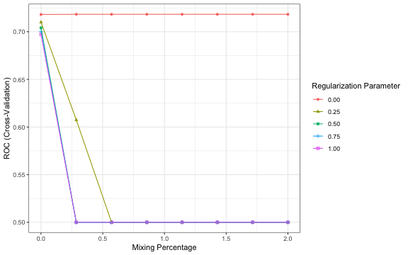

plot of chunk glmnet plots

m.glmnet.bestTune <- m.glmnet$bestTune
save(m.glmnet.bestTune, file="m.glmnet.best.RData")

# Free Memory
rm(m.glmnet)
gc()

##             used   (Mb) gc trigger   (Mb) limit (Mb)   max used   (Mb)
## Ncells   4940755  263.9   31376385 1675.7         NA   57406743 3065.9
## Vcells 451322918 3443.4 1221387127 9318.5      16384 1276946662 9742.4

tune_grid <- expand.grid(
  nrounds = 1000,
  eta = 0.05,
  max_depth = 4,
  gamma = 0,
  colsample_bytree = 1,
  min_child_weight = 9,
  subsample = 1
)

tune_control <- caret::trainControl(
  method = "cv", # cross-validation
  number = 3, # with n folds 
  #index = createFolds(tr_treated$Id_clean), # fix the folds
  verboseIter = FALSE, # no training log
  classProbs = TRUE, # requested the predicted probs (for ROC)
  summaryFunction = twoClassSummary, # needed to produce the ROC/AUC measures
  selectionFunction = "best",
  savePredictions = TRUE, # needed to plot the ROC curves
  allowParallel = TRUE # FALSE for reproducible results 
)

m.xgb <- caret::train(
  default ~., data = lc4_train,
  trControl = tune_control,
  tuneGrid = tune_grid,
  method = "xgbTree",
  verbose = TRUE,
  metric = "ROC"
)

save(m.xgb, file="m.xgb.RData")

lc4_test$pred.xgb <- predict(m.xgb, lc4_test, type ='prob')$yes
lc4_test2$pred.xgb <- predict(m.xgb, lc4_test2, type ='prob')$yes

load("m.xgb.RData")

tuneplot(m.xgb)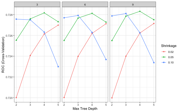

plot of chunk xgb plots

m.xgb.bestTune <- m.xgb$bestTune
save(m.xgb.bestTune, file="m.xgb.best.RData")

# Free Memory
#rm(m.xgb)
gc()

##             used   (Mb) gc trigger   (Mb) limit (Mb)   max used   (Mb)
## Ncells   4686548  250.3   25101108 1340.6         NA   57406743 3065.9
## Vcells 315413285 2406.5  977109702 7454.8      16384 1276946662 9742.4

ctrl <- trainControl(
  method = "cv",
  number = 3, # 3-fold CV
  selectionFunction = "best", # select the best performer
  classProbs = TRUE, # requested the predicted probs (for ROC)
  summaryFunction = twoClassSummary, # needed to produce the ROC/AUC measures
  savePredictions = TRUE, # needed to plot the ROC curves
  allowParallel = FALSE, # set to TRUE to utilize additionl cores (see Ch. 12 but DON'T use w/ ranger!)
  returnData = FALSE, # don't save the training data for each CV iteration -- saves memory
  trim = TRUE, # remove some components of the final model to save memory (may not work with all models)
  verboseIter = TRUE # reports caret's progress
)

grid.ranger <- expand.grid(mtry = c(5, 8),
                      splitrule = c("extratrees"),
                      min.node.size = c(5, 8))

m.ranger <- train(default ~ ., data = lc4_train,
               method = "ranger",
               trControl = ctrl,
               tuneGrid = grid.ranger,
               metric = "ROC")

save(m.ranger, file="m.ranger.RData")

lc4_test$pred.ranger <- predict(m.ranger, lc4_test, type ='prob')$yes
lc4_test2$pred.ranger <- predict(m.ranger, lc4_test2, type ='prob')$yes

load("m.ranger.RData")

tuneplot(m.ranger)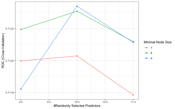

plot of chunk ranger plots

m.ranger.bestTune <- m.ranger$bestTune
save(m.ranger.bestTune, file="m.ranger.best.RData")

# Free Memory
rm(m.ranger)
gc()

##             used   (Mb) gc trigger   (Mb) limit (Mb)   max used   (Mb)
## Ncells  41363089 2209.1   75092641 4010.4         NA   57406743 3065.9
## Vcells 552119064 4212.4  977109702 7454.8      16384 1276946662 9742.4

## Evaluation Next, I evaluate the models based on their performance. I use the metric AUC for that. Poorest performers are the c50 and rpart models. Then logistic and elastic net regression perform pretty well, followed by the ranger model. The best with a test AUC of 0.731 is the gradient boosting model.

roc.glm <- roc(predictor = lc4_test$pred.glm, response = lc4_test$default)
roc.c50 <- roc(predictor = lc4_test$pred.c50, response = lc4_test$default)
roc.rpart <- roc(predictor = lc4_test$pred.rpart, response = lc4_test$default)
roc.glmnet <- roc(predictor = lc4_test$pred.glmnet, response = lc4_test$default)
roc.xgb <- roc(predictor = lc4_test$pred.xgb, response = lc4_test$default)
roc.ranger <- roc(predictor = lc4_test$pred.ranger, response = lc4_test$default)


auc <- c("glm" = round(auc(roc.glm), 3),
         "c50" = round(auc(roc.c50), 3), 
         "rpart" = round(auc(roc.rpart), 3), 
         "glmnet" = round(auc(roc.glmnet), 3),
         "xgb" = round(auc(roc.xgb), 3),
         "ranger" = round(auc(roc.ranger), 3))

g1 <- pROC::ggroc(list(glm=roc.glm,
                       c50 = roc.c50, 
                       xgb=roc.xgb, 
                       ranger=roc.ranger, 
                       rpart=roc.rpart, 
                       glmnet = roc.glmnet)) +
  theme_bw() +
  geom_segment(aes(x = 1, xend = 0, y = 0, yend = 1), color="darkgrey", linetype="dashed")
g1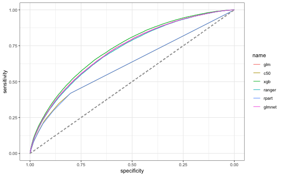

plot of chunk Evaluate

print(auc)

##    glm    c50  rpart glmnet    xgb ranger 
##  0.719  0.620  0.619  0.719  0.731  0.715

Model Stacking

Maybe one model is better in predicting in some dimensions while another models is doing better elsewhere. For this reason I test wheter stacking the models improves performance. I use an elastic net model and feed it with all features and also with the predicted probabilities of the single models (Altough, the model selects only the predicted probabilities to be important). Again I use grid search to find the best parameters.

tune_control <- caret::trainControl(
  method = "cv", # cross-validation
  number = 3, # with n folds
  #index = createFolds(tr_treated$Id_clean), # fix the folds
  verboseIter = FALSE, # no training log
  classProbs = TRUE, # requested the predicted probs (for ROC)
  summaryFunction = twoClassSummary, # needed to produce the ROC/AUC measures
  selectionFunction = "best",
  savePredictions = TRUE, # needed to plot the ROC curves
  allowParallel = TRUE # FALSE for reproducible results
)

grid <- expand.grid(.alpha = seq(0.6, 0.9, length = 7), .lambda = c(0.05, 0.1, 0.15))

m.netstack <- caret::train(
  form = default ~.,
  data = lc4_test,
  trControl = tune_control,
  method = "glmnet",
  metric = "ROC",
  tuneGrid = grid
)

save(m.netstack, file = "m.netstack.RData")

m.netstack.bestTune <- m.netstack$bestTune
save(m.netstack.bestTune, file="m.netstack.best.Rdata")

lc4_test2$pred.netstack <- predict(m.netstack, lc4_test2, type ='prob')$yes

And indeed it is paying off stacking the models. The AUC of the stacked model is with 0.731 a tiny bit higher than the AUC of the gradient boosting model. If we look at the feature importance we see that the only important features are the predictions of the xgb, ranger, glm and glmnet model.

load("m.netstack.RData")
tuneplot(m.netstack)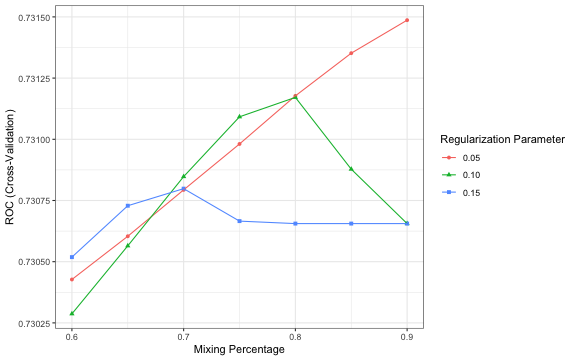

plot of chunk Evaluate Stack

# Free Memory
# rm(m.netstack)
# gc()

roc2.netstack <- roc(predictor = lc4_test2$pred.netstack, response = lc4_test2$default)
roc2.glm <- roc(predictor = lc4_test2$pred.glm, response = lc4_test2$default)
roc2.c50 <- roc(predictor = lc4_test2$pred.c50, response = lc4_test2$default)
roc2.rpart <- roc(predictor = lc4_test2$pred.rpart, response = lc4_test2$default)
roc2.glmnet <- roc(predictor = lc4_test2$pred.glmnet, response = lc4_test2$default)
roc2.xgb <- roc(predictor = lc4_test2$pred.xgb, response = lc4_test2$default)
roc2.ranger <- roc(predictor = lc4_test2$pred.ranger, response = lc4_test2$default)

auc2 <- c("glm" = round(auc(roc2.glm), 3),
         "c50" = round(auc(roc2.c50), 3), 
         "rpart" = round(auc(roc2.rpart), 3), 
         "glmnet" = round(auc(roc2.glmnet), 3),
         "xgb" = round(auc(roc2.xgb), 3),
         "ranger" = round(auc(roc2.ranger), 3),
         "netstack" = round(auc(roc2.netstack), 3))

g2 <- pROC::ggroc(list(xgb=roc2.xgb, stack=roc2.netstack)) +
  theme_bw() +
  geom_segment(aes(x = 1, xend = 0, y = 0, yend = 1), color="darkgrey", linetype="dashed")
g2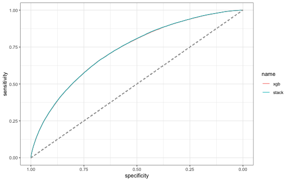

plot of chunk Evaluate Stack

print(auc2)

##      glm      c50    rpart   glmnet      xgb   ranger netstack 
##    0.719    0.618    0.617    0.718    0.730    0.714    0.731

Finally, I train the models with the optimized parameter combination on the full training set and use the stacked model to predict the probabilities of the final test set.

# Model c50
ctrl <- trainControl( # create a caret trainControl object
  method = "cv",
  number = 3, # 3-fold CV
  selectionFunction = "best", # select the best performer
  classProbs = TRUE, # requested the predicted probs (for ROC)
  summaryFunction = twoClassSummary, # needed to produce the ROC/AUC measures
  savePredictions = TRUE, # needed to plot the ROC curves
  allowParallel = TRUE
)

grid <- expand.grid(winnow = FALSE, trials=m.c50.bestTune$trials, model="tree" )

m.c50.final <- train(default ~., 
               data = train,
               method = "C5.0",
               trControl = ctrl,
               tuneGrid = grid,
               metric = "ROC")

load("test_final.RData")
lc4_test_final$pred.c50 <- predict(m.c50.final, lc4_test_final, type ='prob')$yes

# Free Memory
rm(m.c50.final)
gc()

save(lc4_test_final, file="test_final.RData")


# Model Rpart
ctrl <- trainControl( # create a caret trainControl object
  method = "cv",
  number = 3, # 3-fold CV
  selectionFunction = "best", # select the best performer
  classProbs = TRUE, # requested the predicted probs (for ROC)
  summaryFunction = twoClassSummary, # needed to produce the ROC/AUC measures
  savePredictions = TRUE, # needed to plot the ROC curves
  allowParallel = TRUE
)

m.rpart.final <- train(default ~., 
               data = train,
               method = "rpart",
               trControl = ctrl,
               cp=m.rpart.bestTune$cp,
               metric = "ROC")

load("test_final.RData")
lc4_test_final$pred.rpart <- predict(m.rpart.final, lc4_test_final, type ='prob')$yes

# Free Memory
rm(m.rpart.final)
gc()

save(lc4_test_final, file="test_final.RData")


# Model GLM
tune_control <- caret::trainControl(
  method = "cv", # cross-validation
  number = 3, # with n folds 
  verboseIter = FALSE, # no training log
  classProbs = TRUE, # requested the predicted probs (for ROC)
  summaryFunction = twoClassSummary, # needed to produce the ROC/AUC measures
  selectionFunction = "best",
  savePredictions = TRUE, # needed to plot the ROC curves
  allowParallel = TRUE # FALSE for reproducible results 
)

m.glm.final <- caret::train(
  form = default ~., 
  data = train,
  trControl = tune_control,
  method = "glm",
  family = "binomial",
  metric = "ROC"
)

load("test_final.RData")
lc4_test_final$pred.glm <- predict(m.glm.final, lc4_test_final, type ='prob')$yes

# Free Memory
rm(m.glm.final)
gc()

save(lc4_test_final, file="test_final.RData")


# Model glmnet
tune_control <- caret::trainControl(
  method = "cv", # cross-validation
  number = 3, # with n folds 
  #index = createFolds(tr_treated$Id_clean), # fix the folds
  verboseIter = FALSE, # no training log
  classProbs = TRUE, # requested the predicted probs (for ROC)
  summaryFunction = twoClassSummary, # needed to produce the ROC/AUC measures
  selectionFunction = "best",
  savePredictions = TRUE, # needed to plot the ROC curves
  allowParallel = TRUE # FALSE for reproducible results 
)

grid <- expand.grid(.alpha = m.glmnet.bestTune$alpha, .lambda = m.glmnet.bestTune$lambda)

m.glmnet.final <- caret::train(
  form = default ~., 
  data = train,
  trControl = tune_control,
  method = "glmnet",
  metric = "ROC",
  tuneGrid = grid
)

load("test_final.RData")
lc4_test_final$pred.glmnet <- predict(m.glmnet.final, lc4_test_final, type ='prob')$yes

# Free Memory
rm(m.glmnet.final)
gc()

save(lc4_test_final, file="test_final.RData")


# Model XGB
tune_grid <- expand.grid(
  nrounds = m.xgb.bestTune$nrounds,
  eta = m.xgb.bestTune$eta,
  max_depth = m.xgb.bestTune$max_depth,
  gamma = 0,
  colsample_bytree = 1,
  min_child_weight = m.xgb.bestTune$min_child_weight,
  subsample = 1
)

tune_control <- caret::trainControl(
  method = "cv", # cross-validation
  number = 3, # with n folds 
  #index = createFolds(tr_treated$Id_clean), # fix the folds
  verboseIter = FALSE, # no training log
  classProbs = TRUE, # requested the predicted probs (for ROC)
  summaryFunction = twoClassSummary, # needed to produce the ROC/AUC measures
  selectionFunction = "best",
  savePredictions = TRUE, # needed to plot the ROC curves
  allowParallel = TRUE # FALSE for reproducible results 
)

m.xgb.final <- caret::train(
  default ~., data = train,
  trControl = tune_control,
  tuneGrid = tune_grid,
  method = "xgbTree",
  verbose = TRUE,
  metric = "ROC"
)

load("test_final.RData")
lc4_test_final$pred.xgb <- predict(m.xgb.final, lc4_test_final, type ='prob')$yes

# Free Memory
rm(m.xgb.final)
gc()

save(lc4_test_final, file="test_final.RData")


# Model Ranger
ctrl <- trainControl(
  method = "cv",
  number = 3, # 3-fold CV
  selectionFunction = "best", # select the best performer
  classProbs = TRUE, # requested the predicted probs (for ROC)
  summaryFunction = twoClassSummary, # needed to produce the ROC/AUC measures
  savePredictions = TRUE, # needed to plot the ROC curves
  allowParallel = FALSE, # set to TRUE to utilize additionl cores (see Ch. 12 but DON'T use w/ ranger!)
  returnData = FALSE, # don't save the training data for each CV iteration -- saves memory
  trim = TRUE, # remove some components of the final model to save memory (may not work with all models)
  verboseIter = TRUE # reports caret's progress
)

grid.ranger <- expand.grid(mtry = m.ranger.bestTune$mtry,
                      splitrule = m.ranger.bestTune$splitrule,
                      min.node.size = m.ranger.bestTune$min.node.size)

m.ranger.final <- train(default ~ ., data = train,
               method = "ranger",
               trControl = ctrl,
               tuneGrid = grid.ranger,
               metric = "ROC")

load("test_final.RData")
lc4_test_final$pred.ranger <- predict(m.ranger.final, lc4_test_final, type ='prob')$yes

# Free Memory
rm(m.ranger.final)
gc()

save(lc4_test_final, file="test_final.RData")

# Predict Final Value
load("test_final.RData")
lc4_test_final$pred.netstack <- predict(m.netstack, lc4_test_final, type ='prob')$yes
save(lc4_test_final, file="test_final.RData")

Conclusion

I developed a Machine Learning Model to predict loan defaults.
Among the tested models, the xgb algorithm performed best.
However, stacking the models together, improved performance a tiny bit.

load("test_final.RData")

lc4_test_final <- lc4_test_final %>%
  rename(prob = pred.netstack)

# write CSV file to current directory
write.csv(lc4_test_final[c("id", "prob")], "group14.csv", row.names = FALSE)

Predicting the default of lending club loans

Load Data

Feature Engineering

External Data

Topic Modelling

Feature Engineering

Explore Data

Modeling

Model Stacking

Conclusion

Comments You need to have a GitHub Account to comment!

Comments