Creating content from Jupyter notebooks and R markdowns
R Markdown
If you have some Markdowns around, you can use the function below to create jekyll content. Just execute KnitPost(rmd.path) in a R console. Note that you need to add a specific YAML header to your Markdown file.
KnitPost <- function(rmd.path, site.name, basedir="/path/to/basedir/") {
  if(!'package:knitr' %in% search()) library('knitr')

  site.path <- "/pagename"

  ## Some directories.  This will depend on how you organize your page.
  site.path <- site.path # directory of jekyll  (including trailing slash)
  fig.dir <- paste0("public/img/",site.name,"/") # directory to save figures
  posts.path <- paste0(site.path, "_posts/") # directory for converted markdown files
  cache.path <- paste0(site.path, "_cache") # necessary for plots

  render_jekyll(highlight = "pygments")
  opts_knit$set(base.url = "", base.dir = basedir)
  opts_chunk$set(fig.path=fig.dir,
                 fig.width=8,
                 fig.height=5,
                 dev='png',
                 cache=F,
                 warning=F,
                 message=F,
                 cache.path=cache.path,
                 tidy=F)


  out <- paste0(basedir,"_posts/", format(Sys.time(), '%Y-%m-%d-'),basename(gsub(pattern = ".Rmd$", replacement = ".md", x = rmd.path)))

  out.file <- knit(as.character(rmd.path),
                 output = as.character(out),
                 envir = parent.frame(),
                 quiet = T)

  # Correct image paths
  lines <- readLines(as.character(out))
  imglines <- lines[grepl(paste0("public/img/",site.name), lines)]
  split1 <- sapply(strsplit(imglines,"\\("), `[`, 1)
  split2 <- sapply(strsplit(sapply(strsplit(sapply(strsplit(imglines,"\\("), `[`, 2), "/"), `[`, 4), "\\)"),`[`, 1)
  lines[grepl(paste0("public/img/",site.name), lines)] <- paste0(split1, "({{ \"public/img/",site.name,"/", split2, "\" | relative_url }}) ")
  writeLines(lines, as.character(out))
}
The output is between the two horizontal lines below.
This is an R Markdown document. Markdown is a simple formatting syntax for authoring HTML, PDF, and MS Word documents. For more details on using R Markdown see http://rmarkdown.rstudio.com.
When you click the Knit button a document will be generated that includes both content as well as the output of any embedded R code chunks within the document. You can embed an R code chunk like this:
data = read.table("california_highschools.txt", sep = ",", header = T)

head(data)
## School teachers test_score enrollment
## 1 Sunol Glen Unified 10.90 691 195
## 2 Manzanita Elementary 11.15 661 240
## 3 Thermalito Union Elementary 82.90 644 1550
## 4 Golden Feather Union Elementary 14.00 648 243
## 5 Palermo Union Elementary 71.50 641 1335
## 6 Burrel Union Elementary 6.40 606 137x = data$enrollment / data$teachers
y = data$test_score
boxplot(y ~ floor(x))
Jupyter notebooks
Similarly for Jupyter notebooks you can use the following function and execute $ python ipynb_to_jekyll.py notebook.ipynb in a terminal.
#!/usr/bin/env python3
# coding=utf-8
"""
Borrowed and updated from
https://adamj.eu/tech/2014/09/21/using-ipython-notebook-to-write-jekyll-blog-posts/
"""
from __future__ import print_function
from datetime import datetime
import functools
import json
import os
import re
import sys
import io
import base64
def main():
if len(sys.argv) != 2:
print("Usage: {} filename.ipynb".format(sys.argv[0]))
print("Will create filename.md.")
return 1
filename = sys.argv[1]
notebook = json.load(open(filename))
dirname = os.path.dirname(filename)
title = os.path.splitext(os.path.basename(filename))[0]
out_filename = os.path.join(
dirname,
"{}.md".format(title)
)
out_content = ""
mem_file = io.StringIO()
write = functools.partial(print, file=mem_file)
cells = notebook['cells']
now = datetime.now()
write("---")
write("layout: post")
write("title: ")
write("date: ", now.strftime('%Y-%m-%d %H:%M:%S'))
write("---")
xx = 1
for cell in cells:
try:
if cell['cell_type'] == 'markdown':
# Easy
write(''.join(cell['source']))
elif cell['cell_type'] == 'code':
write("{% capture content %}{% highlight python %}")
write(''.join(cell['source']))
write("{% endhighlight %}{% endcapture %}")
write("""{{% include notebook-cell.html execution_count="[{}]:" content=content type='input' %}}""".format(
cell['execution_count'],
))
unknown_types = {o['output_type'] for o in cell['outputs']} - {'stream', 'execute_result', 'display_data'}
if unknown_types:
raise ValueError("Unknown types : {}".format(", ".join(unknown_types)))
for output in cell['outputs']:
if output['output_type'] == 'execute_result':
write("{% capture content %}") #{% highlight python %}")
write(''.join(output['data']["text/html"])) #plain
write("{% endcapture %}") #{% endhighlight %}
write(
"""{{% include notebook-cell.html execution_count="[{}]:" "
"content=content type='output' %}}""".format(
cell['execution_count'],
)
)
elif output['output_type'] == 'display_data':
png_b64text = output['data']["image/png"]
bpng_b64text = bytes(png_b64text, encoding="UTF-8")
with open("image" + str(xx) + ".png", "wb") as fh:
fh.write(base64.decodestring(bpng_b64text))
#png_recovered = base64.decodestring(png_b64text) #this worked under python 2.
#f = open("img.png", "w")
#f.write(png_recovered)
fh.close()
write(" + ".png | relative_url }})")
xx += 1
else:
write("""<pre class="stream">""")
if output['output_type'] == 'stream':
write(''.join(output['text']).strip(" \n")) #text
elif output['output_type'] == 'pyerr':
write('\n'.join(strip_colors(o)
for o in output['traceback']).strip(" \n"))
write("</pre>")
except:
print(cell, type(cell))
raise
write("")
with open(out_filename, "w") as out_file:
out_file.write(mem_file.getvalue())
print("{} created.".format(out_filename))
ansi_escape = re.compile(r'\x1b[^m]*m')
def strip_colors(string):
return ansi_escape.sub('', string)
if __name__ == '__main__':
main()
Finally we need some scss styling for the page in addition to the standard syntax highlighter:
 div.cell {
    background-color: var(--code-background-color);
     border-radius: 5px;
     padding: 5px;
    page-break-inside: auto;
    display: -webkit-box;
    -webkit-box-orient: horizontal;
    -webkit-box-align: stretch;
    display: -moz-box;
    -moz-box-orient: horizontal;
    -moz-box-align: stretch;
    display: box;
    box-orient: horizontal;
    box-align: stretch;
    display: flex;
    flex-direction: row;
    align-items: stretch;
    /*overflow-x: auto;*/
   /* border: 1px dashed #444; */
}


.prompt {
  min-width: 10ex;
  padding: 0em;
  margin: 0px 3px 0px 0px;
  font-family: monospace;
  font-size: 14px;
  text-align: left;
  line-height: 1.21429em;
  -webkit-touch-callout: none;
  -webkit-user-select: none;
  -khtml-user-select: none;
  -moz-user-select: none;
  -ms-user-select: none;
  user-select: none;
  cursor: default;
 white-space: nowrap;
}

div.prompt {
  &.input-prompt {
    color: #303F9F;
    /*border-top: 1px solid transparent;*/
  }
  &.output-prompt {
    color: #D84315;
  }
}

pre.stream {
    font-family: 'Lucida Console', 'Monaco', monospace;
    font-size: 11px;
    color: #808080;
    line-height: 1.2;
    background-color: var(--background-color);;
    padding: 0rem 0rem 0rem 1rem;
    overflow-x: auto;
   /* white-space: pre-wrap !important;  CSS 2.1 */
  }

  blockquote {
    color: #aaa;
    padding-left: 10px;
    border-left: 1px dotted #666;
  }
Below is the output of this function
from pylab import *
import numpy as np
import pandas as pdx = np.linspace(0, 5, 10)
xx = np.linspace(-0.75, 1., 100)
n = np.array([0,1,2,3,4,5])
dates = pd.date_range('20130101', periods=6)
df = pd.DataFrame(np.random.randn(6,4), index=dates, columns=list('ABCD'))
df| A | B | C | D | |
|---|---|---|---|---|
| 2013-01-01 | 2.278744 | -0.652785 | 0.574983 | -0.408235 |
| 2013-01-02 | 0.886904 | -1.415350 | 0.487806 | -0.117535 |
| 2013-01-03 | 1.280152 | 0.451589 | 2.450064 | -0.159981 |
| 2013-01-04 | -0.163132 | 0.141542 | 1.810313 | 2.263799 |
| 2013-01-05 | -0.488827 | 0.263963 | 0.598489 | 0.933941 |
| 2013-01-06 | -1.589058 | 0.054630 | 1.425882 | 0.133386 |
This is an example text.
fig, axes = plt.subplots(1, 4, figsize=(12,3))

axes[0].scatter(xx, xx + 0.25*np.random.randn(len(xx)))
axes[0].set_title("scatter")

axes[1].step(n, n**2, lw=2)
axes[1].set_title("step")

axes[2].bar(n, n**2, align="center", width=0.5, alpha=0.5)
axes[2].set_title("bar")

axes[3].fill_between(x, x**2, x**3, color="green", alpha=0.5);
axes[3].set_title("fill_between");
show(fig)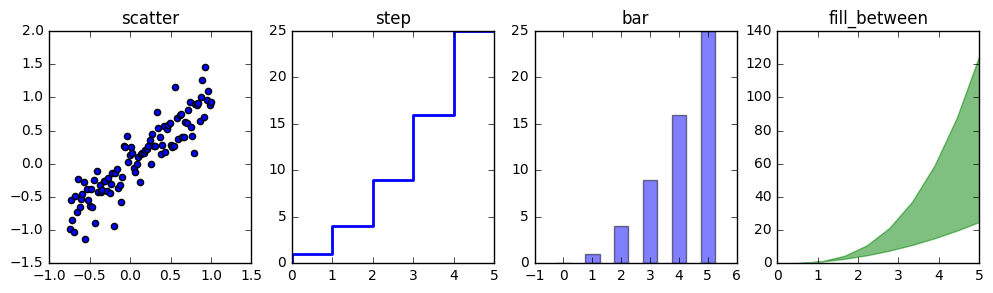
# polar plot using add_axes and polar projection
fig = plt.figure()
ax = fig.add_axes([0.0, 0.0, .6, .6], polar=True)
t = np.linspace(0, 2 * np.pi, 100)
ax.plot(t, t, color='blue', lw=3);
show(fig)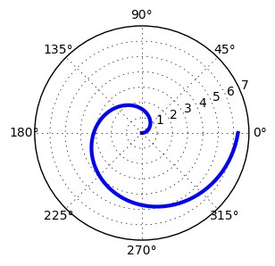
Comments You need to have a GitHub Account to comment!
Post comment