Forecasting Swiss GDP Growth after the SNB abandoned the exchange rate floor
“The only function of economic forecasting is to make astrology look respectable.” 1
Since economic output represents the aggregated activity of many agents, influenced by forces seen and unseen, it is a wonder forecasters ever get it right. Nevertheless, I try to forecast Swiss GDP growth after an appreciation of 15% of the CHF vis-à-vis the EUR as it was the case when the SNB repealed the minimum rate.2 To do this, I use an ARMAX and a VARMAX model. The models predict considerably lower GDP growth which confirms that the models reflect the negative relationship between GDP growth and the exchange rate. Hence, both types of models exhibit quite reasonable predictive power.
To estimate the models, I use the SARIMAX and the VARMAX routines of Statsmodels. The data used can be found on the database of the St. Louis Fred and the OECD. The VARMAX model contains Swiss GDP growth, inflation, unemployment rate, exports growth, a shorter and a longer yield spread. Lagged GDP of the Euro Area and lagged CHF/EUR exchangerate build the exogenous data block. Granger Causality tests show that from a statistically point of view it’s justified to treat the exchange rate as exogenous which is an assumption that is often used when forecasting GDP growth in a small open economy, although it does not make a lot of sense economically. Economically it can reasonably be assumed, however, that Euro Area GDP growth is exogenous to Swiss GDP growth because Switzerland is a small open economy and thus is unlikely to affect GDP growth in the EU.
import numpy as np
import pandas as pd
import statsmodels.api as sm
from pandas.io.data import DataReader
import matplotlib.pyplot as plt
import warnings
warnings.simplefilter('ignore')
/anaconda/lib/python3.5/site-packages/pandas/io/data.py:35: FutureWarning: The pandas.io.data module is moved to a separate package (pandas-datareader) and will be removed from pandas in a future version. After installing the pandas-datareader package (https://github.com/pydata/pandas-datareader), you can change the import ``from pandas.io import data, wb`` to ``from pandas_datareader import data, wb``. FutureWarning)
table = pd.read_excel('forecasting_data.xlsx')
idx = table.observation_date
data = table[['SwissGDP','Inflation','Unemployment','Exports','Shortspread','Longspread']]
data.index=idx
xdata = table[['EUR/CHF','EUR/CHF_L1','EUR/CHF_L2','EUR/CHF_L3','EuroGDP_L1']]
xdata.index=idx
SwissGDP = data[['SwissGDP']]

fig1 = plt.figure(figsize=(8,5))
ax1 = fig1.add_subplot(211)
fig = sm.graphics.tsa.plot_acf(SwissGDP, lags=6, ax=ax1)
ax2 = fig1.add_subplot(212)
fig1 = sm.graphics.tsa.plot_pacf(SwissGDP, lags=6, ax=ax2)
plt.show(fig1)
The figure above shows the ACF and the PACF of Swiss GDP growth. The ACF is significantly different from zero up to two lags while the PACF is only significantly different from zero for lag one. Therefore, p = 4 and q = 4 should be according to Box and Jenkins (1976) an appropriate maximum order for the ARMAX(p,q) model. In an automated procedure several information criteria are calculated to trade-off explanatory power with parsimony.
aic = pd.DataFrame(np.zeros((5,5), dtype=float))
bic = pd.DataFrame(np.zeros((5,5), dtype=float))

# Iterate over all ARMA(p,q) models with p,q in [0,]
for p in range(5):
    for q in range(5):
        if p == 0 and q == 0:
            continue

        # Estimate the model with no missing datapoints
        mod = sm.tsa.statespace.SARIMAX(SwissGDP, xdata, order=(p,0,q), enforce_invertibility=True)
        try:
            res = mod.fit(maxiter=5000, disp = False)
            aic.iloc[p,q] = res.aic
            bic.iloc[p,q] = res.bic
        except:
            aic.iloc[p,q] = np.nan
            bic.iloc[p,q] = np.nan

aic.iloc[0,0] = np.nan
bic.iloc[0,0] = np.nan

print(aic)
print(bic)

q = aic.min().idxmin()
p = aic.idxmin()[q]
0           1           2           3           4
0         NaN  264.613956  265.895288  263.718360  265.311417
1  262.245898  255.756811  251.495686  255.245270  257.234556
2  262.613856         NaN         NaN  255.466728  256.541741
3  261.917222  263.947968         NaN         NaN         NaN
4  263.823613  265.827257         NaN         NaN         NaN
            0           1           2           3           4
0         NaN  285.155274  289.371079  290.128625  294.656156
1  282.787215  279.232602  277.905952  284.590009  289.513770
2  286.089647         NaN         NaN  287.745941  291.755428
3  288.327487  293.292707         NaN         NaN         NaN
4  293.168352  298.106470         NaN         NaN         NaN
The AIC and the BIC are both minimized for \(p = 1\) and \(q = 2\), therefore an ARMAX(1,2) model is used here.
ARMA model
Due to Wold (1938), a covariance-stationary equation can be written as the so-called “Wold-Decomposition”:
\[\begin{aligned} Y_t = \mu + \sum_{j=0}^{\infty} \psi_j \epsilon_{t-j} \end{aligned}\]where \(\epsilon_t\) is the error from forecasting \(Y_t\) solely with lagged values of \(Y_t\). A Wold representation in principle requires fitting an infinite number of parameters (\(\psi_1, \psi_2, ...\)). With a finite number of observations this will never be possible. However, in practice a typical assumption is that \(Y_t\) is a causal process and \(\psi(L)\) can be approximated from its causal representation:
\[\begin{aligned} \sum_{j=0}^\infty \psi_j L^j = \frac{\Theta(L)}{\Phi(L)} \equiv \frac{(1 + \theta_1L + \theta_2L^2 + ... + \theta_qL^q)}{(1 - \phi_1L - \phi_2L^2 - ... - \phi_pL^p)} \end{aligned}\]ARMA modelling seeks a finite parameter approximation to the Wold representation. Box and Jenkins (1976) emphasise parsimony in the choice of the AR order \(p\) and the MA \(q\) order
The general ARMA model is:
\[\begin{aligned} Y_t = \sum_{i=0}^p \phi_i Y_{t-i} + \epsilon_t + \sum_{j=0}^q \theta_j \epsilon_{t-j} \end{aligned}\]where \(\epsilon_t\) is a disturbance term(white noise) and \(Y_t\) is the stationary forecast variable. The typical strategy implies:
- Select an appropriate maximum \(p, q\) order for the ARMA (p, q) model.
- Estimate \(\phi(L)\) and \(\theta(L)\) associated with each choice of \(p\) and \(q\).
- Select the best model (choice of \(p\) and \(q\)) based on model diagnostics.
# Statespace
mod = sm.tsa.statespace.SARIMAX(SwissGDP, xdata, order=(p,0,q))
res = mod.fit(maxiter=5000)
fig2 = res.plot_diagnostics()
print(res.summary())
plt.show(fig2)
Statespace Model Results
==============================================================================
Dep. Variable:               SwissGDP   No. Observations:                  139
Model:               SARIMAX(1, 0, 2)   Log Likelihood                -116.748
Date:                Thu, 05 Jan 2017   AIC                            251.496
Time:                        17:11:42   BIC                            277.906
Sample:                    04-01-1980   HQIC                           262.228
                         - 10-01-2014
Covariance Type:                  opg
==============================================================================
                 coef    std err          z      P>|z|      [0.025      0.975]
------------------------------------------------------------------------------
EUR/CHF        0.0316      0.021      1.535      0.125      -0.009       0.072
EUR/CHF_L1     0.0415      0.026      1.609      0.108      -0.009       0.092
EUR/CHF_L2     0.0575      0.026      2.194      0.028       0.006       0.109
EUR/CHF_L3     0.0512      0.020      2.589      0.010       0.012       0.090
EuroGDP_L1     0.3566      0.095      3.740      0.000       0.170       0.544
ar.L1          0.9989      0.004    272.166      0.000       0.992       1.006
ma.L1         -0.7317      0.096     -7.607      0.000      -0.920      -0.543
ma.L2         -0.2350      0.093     -2.529      0.011      -0.417      -0.053
sigma2         0.3097      0.035      8.910      0.000       0.242       0.378
===================================================================================
Ljung-Box (Q):                       30.26   Jarque-Bera (JB):                34.75
Prob(Q):                              0.87   Prob(JB):                         0.00
Heteroskedasticity (H):               0.45   Skew:                            -0.01
Prob(H) (two-sided):                  0.01   Kurtosis:                         5.45
===================================================================================

Warnings:
[1] Covariance matrix calculated using the outer product of gradients (complex-step).
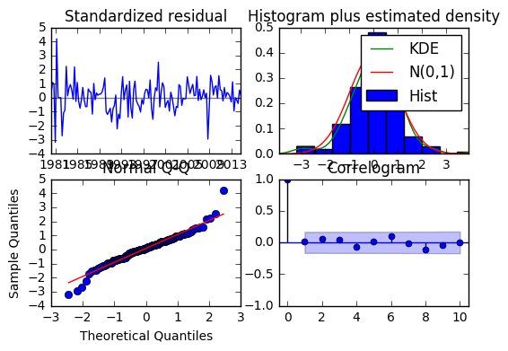
The residual plot suggest that the ARMA model fits pretty well. The fitted values track the actual values and even cover the recession during the financial crisis. The residuals look reasonably independent and identically distributed according to the ACF and also resemble a normal distribution. By looking at the ACF of the residuals it’s observable that there are no lags which are autocorrelated.
Next, the exogenous variables for the forecasting task are generated. For simplicity, I assume that the exchange rate decreases by 15% in 2015Q1 (due to the decision of the SNB to repeal the euro minimum rate on January 15) and is zero otherwise. The lagged Euro Area GDP is set to it’s mean. Then the model is used to forecast 12 quarters ahead.
# Generate Exogenous Data for Forecasting
fx = pd.DataFrame(index=list(range(0, 12)) , columns=xdata.columns)
fx = fx.fillna(0)
fx.iloc[0,0] = -15.00
fx.iloc[1,1] = -15.00
fx.iloc[2,2] = -15.00
fx.iloc[3,3] = -15.00

fx.iloc[0:12,4] = np.mean(xdata[['EuroGDP_L1']]).values# In-sample one-step-ahead predictions, and out-of-sample forecasts
nforecast = 11
predict = res.get_prediction(end=mod.nobs + nforecast, exog = fx)
""" idx = np.arange(len(predict.predicted_mean)) """
predict_ci90 = predict.conf_int(alpha=0.1)
predict_ci60 = predict.conf_int(alpha=0.4)
predict_ci30 = predict.conf_int(alpha=0.7)
fidx = predict_ci90.index
predict_ci90.iloc[138,:] = SwissGDP.iloc[138,:].values
predict_ci60.iloc[138,:] = SwissGDP.iloc[138,:].values
predict_ci30.iloc[138,:] = SwissGDP.iloc[138,:].values
# Graph
fig3, ax = plt.subplots(figsize=(12,6))
ax.grid()
ax.plot(idx,SwissGDP,'k',label='', alpha=0.7, linewidth=0.75)
ax.plot(idx,SwissGDP,'k.', label='Actual Values', alpha=0.7, linewidth=0.75)
# Plot
ax.plot( predict.predicted_mean[:-nforecast-1], 'gray',label='In Sample Prediction')
ax.plot(fidx[-nforecast-1:], predict.predicted_mean[-nforecast-1:], 'k--', linestyle='--', linewidth=1.5,label='Out of Sample Prediction')
ax.fill_between(fidx[-nforecast-2:], predict_ci90.iloc[-nforecast-2:, 0], predict_ci90.iloc[-nforecast-2:, 1], alpha=0.15, label= '')
ax.fill_between(fidx[-nforecast-2:], predict_ci60.iloc[-nforecast-2:, 0], predict_ci60.iloc[-nforecast-2:, 1], alpha=0.15, label= '')
ax.fill_between(fidx[-nforecast-2:], predict_ci30.iloc[-nforecast-2:, 0], predict_ci30.iloc[-nforecast-2:, 1], alpha=0.15, label= '')
# Retrieve and also plot the NBER recession indicators
rec = DataReader('USREC', 'fred', start=idx[0], end=idx[138])
recr = rec.iloc[0:413:3,0]
ylim = ax.get_ylim()
ax.fill_between(recr.index, ylim[0], ylim[1], recr, facecolor='k', alpha=0.1);
ax.legend()
ax.set_xlim(730000.0, 736603.0)
ax.set(title='ARMAX - Forecasting Swiss GDP');
plt.show(fig3)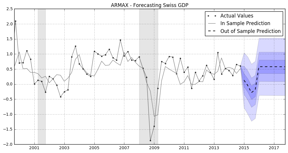
We see this scenario predicts Swiss GDP to be considerably lower because of the appreciation. This reflects the positive relationship between a depreciation and GDP growth. Therefore, an appreciation of the swiss franc vis-à-vis the euro leads to lower Swiss GDP growth.
VAR model
A VAR(p) process in reduced form is:
\[\begin{aligned} y_t = c + \Phi_1y_{t-1} + ... + \Phi_py_{t-p} + \epsilon_t \end{aligned}\]Here \(y_t\) represents a set of variables collected in a vector, c denotes a vector of constants, \(\Phi_j\) a matrix of autoregressive coefficients and \(\epsilon_t\) is white noise. Since the parameters of \(\Phi_j\) are unknown, we have to estimate these parameters. To do so, the VAR can be represented in companion form:
\[\begin{aligned} Y &= (y_1, y_2, ... , y_T) \\[2em] B &= (c, \Phi_1, \Phi_2, ... , \Phi_p) \\[2em] Z &= \left[\begin{array}{cccc} 1 & 1 & ... & 1 \\ y_{0} & y_1 & ... & y_{T-1} \\ \vdots & \vdots & \ddots & \vdots \\ y_{-p+1} & y_{-p+2} & ... & y_{T-p} \end{array} \right] \\[3em] U &= (\epsilon_1, \epsilon_2, ... , \epsilon_T) \end{aligned}\]The VAR(p) can now be written compactly as
\[\begin{aligned} Y = BZ + U \end{aligned}\]and coefficients can easily be estimated via OLS or Maximum Likelihood.
# Iterate over all VARMAX(p,q) models with p,q in [0,]
for p in  range(5):
    for q in  range(5):
        if p == 0 and q == 0:
            continue

        # Estimate the model with no missing datapoints
        mod = sm.tsa.VARMAX(data, xdata, order=(p,q), enforce_invertibility=True)
        try:
            res = mod.fit(maxiter=100, disp = False)
            aic.iloc[p,q] = res.aic
            bic.iloc[p,q] = res.bic
        except:
            aic.iloc[p,q] = np.nan
            bic.iloc[p,q] = np.nan

aic.iloc[0,0] = np.nan
bic.iloc[0,0] = np.nan

print(aic)
print(bic)

q = aic.min().idxmin()
p = aic.idxmin()[q]
0            1            2            3            4
0          NaN  2327.172822  2268.377277  2268.557987  2184.283078
1  1738.137507  1671.993551  1703.809500  1755.831867  1725.441905
2  1595.173709  1697.197868  1720.744466  1837.434508  1814.274102
3  1691.637533  1675.031941  1755.366443  1863.706566  1953.631488
4  1709.367598  1702.215088  1805.406073  1898.357519  1983.406628
             0            1            2            3            4
0          NaN  2600.078897  2646.924414  2752.746186  2774.112339
1  2011.043582  2050.540689  2187.997699  2345.661128  2420.912227
2  1973.720847  2181.386067  2310.573727  2532.904830  2615.385485
3  2175.825732  2264.861201  2450.836765  2664.817950  2860.383933
4  2299.196858  2397.685410  2606.517457  2805.109964  2995.800135
Both information criteria are minimized within the VARMAX(2,0) model.
# Statespace
mod = sm.tsa.VARMAX(data, xdata, order=(p,q), enforce_invertibility=True)
res = mod.fit(maxiter=5000, disp = False)
fig4 = res.plot_diagnostics(0)
print(res.summary())
plt.show(fig4)
Statespace Model Results ============================================================================================================================================= Dep. Variable: ['SwissGDP', 'Inflation', 'Unemployment', 'Exports', 'Shortspread', 'Longspread'] No. Observations: 139 Model: VARX(2) Log Likelihood -666.505 + intercept AIC 1591.009 Date: Mon, 09 Jan 2017 BIC 1969.556 Time: 23:08:04 HQIC 1744.841 Sample: 04-01-1980 - 10-01-2014 Covariance Type: opg ================================================================================================================================= Ljung-Box (Q): 33.70, 98.21, 41.30, 35.91, 34.08, 103.01 Jarque-Bera (JB): 19.32, 0.06, 211.33, 33.69, 111.01, 15.63 Prob(Q): 0.75, 0.00, 0.41, 0.66, 0.73, 0.00 Prob(JB): 0.00, 0.97, 0.00, 0.00, 0.00, 0.00 Heteroskedasticity (H): 0.78, 0.86, 2.87, 1.16, 0.08, 0.20 Skew: -0.38, 0.04, -0.69, 0.44, 1.24, 0.16 Prob(H) (two-sided): 0.41, 0.61, 0.00, 0.62, 0.00, 0.00 Kurtosis: 4.66, 2.94, 8.88, 5.25, 6.61, 4.61 Results for equation SwissGDP =================================================================================== coef std err z P>|z| [0.025 0.975] ----------------------------------------------------------------------------------- const 0.2912 0.851 0.342 0.732 -1.376 1.959 L1.SwissGDP 0.2160 0.593 0.364 0.716 -0.947 1.379 L1.Inflation 0.0502 0.377 0.133 0.894 -0.689 0.789 L1.Unemployment 0.2273 1.157 0.196 0.844 -2.041 2.495 L1.Exports 0.0265 0.042 0.629 0.530 -0.056 0.109 L1.Shortspread -0.1068 0.459 -0.233 0.816 -1.006 0.792 L1.Longspread -0.2581 0.549 -0.470 0.638 -1.334 0.818 L2.SwissGDP -0.0129 0.453 -0.028 0.977 -0.900 0.874 L2.Inflation -0.1513 0.376 -0.403 0.687 -0.888 0.585 L2.Unemployment -0.2115 1.189 -0.178 0.859 -2.542 2.119 L2.Exports -0.0023 0.073 -0.031 0.975 -0.145 0.141 L2.Shortspread 0.1188 0.549 0.217 0.829 -0.957 1.194 L2.Longspread 0.3291 0.604 0.545 0.586 -0.855 1.514 beta.EUR/CHF -0.0030 0.135 -0.023 0.982 -0.268 0.262 beta.EUR/CHF_L1 0.0634 0.105 0.602 0.547 -0.143 0.270 beta.EUR/CHF_L2 0.0287 0.100 0.287 0.774 -0.167 0.225 beta.EUR/CHF_L3 -0.0029 0.147 -0.020 0.984 -0.292 0.286 beta.EuroGDP_L1 0.1038 0.632 0.164 0.870 -1.134 1.342 Results for equation Inflation =================================================================================== coef std err z P>|z| [0.025 0.975] ----------------------------------------------------------------------------------- const 0.3652 0.677 0.539 0.590 -0.963 1.693 L1.SwissGDP 0.0388 0.418 0.093 0.926 -0.781 0.859 L1.Inflation -0.2694 0.393 -0.686 0.493 -1.039 0.500 L1.Unemployment 0.4424 1.403 0.315 0.753 -2.308 3.193 L1.Exports 0.0146 0.043 0.342 0.732 -0.069 0.099 L1.Shortspread 0.0660 0.453 0.146 0.884 -0.822 0.954 L1.Longspread -0.1757 0.595 -0.295 0.768 -1.343 0.991 L2.SwissGDP -0.2069 0.575 -0.360 0.719 -1.335 0.921 L2.Inflation 0.1265 0.222 0.571 0.568 -0.308 0.561 L2.Unemployment -0.4376 1.384 -0.316 0.752 -3.150 2.274 L2.Exports 0.0027 0.055 0.050 0.960 -0.105 0.110 L2.Shortspread 0.2494 0.382 0.652 0.514 -0.500 0.999 L2.Longspread -0.0575 0.631 -0.091 0.927 -1.294 1.180 beta.EUR/CHF 0.0039 0.087 0.044 0.965 -0.166 0.174 beta.EUR/CHF_L1 0.0026 0.127 0.021 0.983 -0.246 0.251 beta.EUR/CHF_L2 0.0177 0.109 0.163 0.871 -0.195 0.231 beta.EUR/CHF_L3 0.0306 0.104 0.296 0.768 -0.172 0.234 beta.EuroGDP_L1 0.2990 0.544 0.550 0.582 -0.767 1.365 Results for equation Unemployment =================================================================================== coef std err z P>|z| [0.025 0.975] ----------------------------------------------------------------------------------- const 0.1599 0.148 1.079 0.280 -0.130 0.450 L1.SwissGDP -0.0638 0.091 -0.703 0.482 -0.242 0.114 L1.Inflation 0.0056 0.108 0.052 0.959 -0.206 0.217 L1.Unemployment 1.7436 0.185 9.450 0.000 1.382 2.105 L1.Exports 0.0018 0.011 0.167 0.867 -0.019 0.022 L1.Shortspread 0.0004 0.068 0.006 0.995 -0.132 0.133 L1.Longspread 0.0164 0.142 0.115 0.908 -0.262 0.294 L2.SwissGDP -0.0145 0.131 -0.111 0.912 -0.271 0.242 L2.Inflation 0.0060 0.078 0.077 0.939 -0.147 0.159 L2.Unemployment -0.7866 0.191 -4.122 0.000 -1.161 -0.413 L2.Exports 0.0034 0.014 0.247 0.805 -0.023 0.030 L2.Shortspread -0.0339 0.094 -0.362 0.718 -0.217 0.150 L2.Longspread -0.0070 0.134 -0.052 0.959 -0.271 0.257 beta.EUR/CHF -0.0009 0.015 -0.065 0.948 -0.029 0.028 beta.EUR/CHF_L1 -0.0027 0.014 -0.195 0.846 -0.029 0.024 beta.EUR/CHF_L2 0.0017 0.019 0.092 0.927 -0.035 0.039 beta.EUR/CHF_L3 0.0046 0.016 0.296 0.767 -0.026 0.035 beta.EuroGDP_L1 -0.0270 0.141 -0.192 0.848 -0.303 0.249 Results for equation Exports =================================================================================== coef std err z P>|z| [0.025 0.975] ----------------------------------------------------------------------------------- const 0.2117 8.834 0.024 0.981 -17.103 17.527 L1.SwissGDP 1.4168 7.507 0.189 0.850 -13.297 16.131 L1.Inflation -0.1542 3.754 -0.041 0.967 -7.512 7.203 L1.Unemployment 4.2236 15.231 0.277 0.782 -25.629 34.076 L1.Exports -0.2334 0.328 -0.711 0.477 -0.877 0.410 L1.Shortspread 0.0022 3.357 0.001 0.999 -6.577 6.581 L1.Longspread -1.9147 4.632 -0.413 0.679 -10.993 7.164 L2.SwissGDP -0.0285 5.307 -0.005 0.996 -10.430 10.373 L2.Inflation -1.3139 3.632 -0.362 0.718 -8.432 5.804 L2.Unemployment -4.0944 13.846 -0.296 0.767 -31.232 23.043 L2.Exports -0.1999 0.380 -0.527 0.598 -0.944 0.544 L2.Shortspread 0.9305 4.161 0.224 0.823 -7.225 9.086 L2.Longspread 2.1317 4.209 0.507 0.613 -6.117 10.380 beta.EUR/CHF 0.0228 1.173 0.019 0.985 -2.277 2.323 beta.EUR/CHF_L1 0.1065 1.216 0.088 0.930 -2.278 2.491 beta.EUR/CHF_L2 0.1484 0.769 0.193 0.847 -1.358 1.655 beta.EUR/CHF_L3 -0.1000 0.723 -0.138 0.890 -1.517 1.317 beta.EuroGDP_L1 1.7469 4.490 0.389 0.697 -7.053 10.546 Results for equation Shortspread =================================================================================== coef std err z P>|z| [0.025 0.975] ----------------------------------------------------------------------------------- const 0.1305 1.601 0.082 0.935 -3.008 3.269 L1.SwissGDP -0.0318 0.960 -0.033 0.974 -1.914 1.851 L1.Inflation 0.0794 1.156 0.069 0.945 -2.187 2.346 L1.Unemployment 0.5326 2.243 0.237 0.812 -3.864 4.929 L1.Exports -0.0027 0.153 -0.018 0.986 -0.303 0.297 L1.Shortspread 0.3506 0.523 0.671 0.503 -0.674 1.375 L1.Longspread -0.0849 1.719 -0.049 0.961 -3.454 3.285 L2.SwissGDP 0.5461 1.114 0.490 0.624 -1.637 2.729 L2.Inflation 0.1820 1.366 0.133 0.894 -2.495 2.859 L2.Unemployment -0.5416 2.317 -0.234 0.815 -5.082 3.999 L2.Exports -0.0243 0.118 -0.205 0.837 -0.256 0.207 L2.Shortspread 0.0617 0.583 0.106 0.916 -1.081 1.204 L2.Longspread 0.0132 1.674 0.008 0.994 -3.269 3.295 beta.EUR/CHF -0.0138 0.183 -0.075 0.940 -0.372 0.345 beta.EUR/CHF_L1 -0.0377 0.225 -0.168 0.867 -0.479 0.403 beta.EUR/CHF_L2 -0.0057 0.186 -0.030 0.976 -0.369 0.358 beta.EUR/CHF_L3 -0.0228 0.217 -0.105 0.916 -0.448 0.402 beta.EuroGDP_L1 -0.2505 0.822 -0.305 0.761 -1.861 1.360 Results for equation Longspread =================================================================================== coef std err z P>|z| [0.025 0.975] ----------------------------------------------------------------------------------- const 0.0375 0.840 0.045 0.964 -1.609 1.684 L1.SwissGDP -0.0971 0.480 -0.202 0.840 -1.038 0.844 L1.Inflation -0.1951 0.422 -0.463 0.644 -1.022 0.632 L1.Unemployment -0.0719 1.781 -0.040 0.968 -3.562 3.418 L1.Exports 0.0058 0.048 0.122 0.903 -0.087 0.099 L1.Shortspread 0.2619 0.321 0.816 0.415 -0.367 0.891 L1.Longspread 1.1997 0.611 1.962 0.050 0.001 2.398 L2.SwissGDP 0.0101 0.593 0.017 0.986 -1.151 1.171 L2.Inflation -0.0314 0.320 -0.098 0.922 -0.658 0.595 L2.Unemployment 0.1315 1.703 0.077 0.938 -3.205 3.468 L2.Exports -0.0018 0.074 -0.024 0.981 -0.147 0.143 L2.Shortspread -0.2239 0.300 -0.747 0.455 -0.811 0.363 L2.Longspread -0.3825 0.557 -0.687 0.492 -1.474 0.709 beta.EUR/CHF 0.0040 0.159 0.025 0.980 -0.308 0.316 beta.EUR/CHF_L1 -0.0169 0.154 -0.110 0.913 -0.319 0.285 beta.EUR/CHF_L2 -0.0314 0.077 -0.406 0.684 -0.183 0.120 beta.EUR/CHF_L3 0.0078 0.141 0.055 0.956 -0.269 0.285 beta.EuroGDP_L1 0.0081 0.590 0.014 0.989 -1.147 1.164 Error covariance matrix ===================================================================================================== coef std err z P>|z| [0.025 0.975] ----------------------------------------------------------------------------------------------------- sqrt.var.SwissGDP 0.5079 0.124 4.107 0.000 0.265 0.750 sqrt.cov.SwissGDP.Inflation 0.0564 0.171 0.330 0.742 -0.279 0.392 sqrt.var.Inflation 0.4902 0.125 3.935 0.000 0.246 0.734 sqrt.cov.SwissGDP.Unemployment -0.0192 0.043 -0.452 0.651 -0.103 0.064 sqrt.cov.Inflation.Unemployment 0.0051 0.056 0.092 0.926 -0.104 0.114 sqrt.var.Unemployment 0.0825 0.017 4.847 0.000 0.049 0.116 sqrt.cov.SwissGDP.Exports 1.4706 2.281 0.645 0.519 -3.000 5.941 sqrt.cov.Inflation.Exports 0.5989 2.527 0.237 0.813 -4.354 5.551 sqrt.cov.Unemployment.Exports 0.1911 2.621 0.073 0.942 -4.946 5.329 sqrt.var.Exports 3.9067 1.106 3.533 0.000 1.739 6.074 sqrt.cov.SwissGDP.Shortspread -0.0485 0.680 -0.071 0.943 -1.382 1.285 sqrt.cov.Inflation.Shortspread 0.0111 0.426 0.026 0.979 -0.825 0.847 sqrt.cov.Unemployment.Shortspread -0.0115 0.719 -0.016 0.987 -1.420 1.397 sqrt.cov.Exports.Shortspread 0.0584 0.337 0.173 0.863 -0.603 0.719 sqrt.var.Shortspread 0.7694 0.278 2.767 0.006 0.224 1.314 sqrt.cov.SwissGDP.Longspread -0.0693 0.222 -0.313 0.754 -0.503 0.365 sqrt.cov.Inflation.Longspread -0.0595 0.168 -0.354 0.723 -0.389 0.270 sqrt.cov.Unemployment.Longspread -0.0262 0.376 -0.070 0.945 -0.764 0.711 sqrt.cov.Exports.Longspread -0.0238 0.242 -0.098 0.922 -0.498 0.451 sqrt.cov.Shortspread.Longspread -0.0599 0.189 -0.316 0.752 -0.431 0.311 sqrt.var.Longspread 0.3893 0.135 2.883 0.004 0.125 0.654 ===================================================================================================== Warnings: [1] Covariance matrix calculated using the outer product of gradients (complex-step).
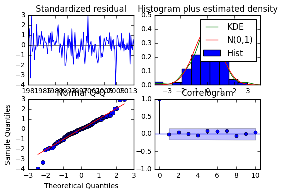
The residual diagnostics plot looks quite similar to the one of the ARMAX model.
Also the VARMAX model predicts the GDP to be considerably lower.
# In-sample one-step-ahead predictions, and out-of-sample forecasts
nforecast = 11
predict = res.get_prediction(end=mod.nobs + nforecast, exog = fx)
""" idx = np.arange(len(predict.predicted_mean)) """
predict_ci90 = predict.conf_int(alpha=0.1)
predict_ci60 = predict.conf_int(alpha=0.4)
predict_ci30 = predict.conf_int(alpha=0.7)
fidx = predict_ci90.index
predict_ci90.iloc[138,:] = SwissGDP.iloc[138,:].values
predict_ci60.iloc[138,:] = SwissGDP.iloc[138,:].values
predict_ci30.iloc[138,:] = SwissGDP.iloc[138,:].values

# Graph
fig5, ax = plt.subplots(figsize=(12,6))
ax.grid()
ax.plot(idx,SwissGDP,'k',label='', alpha=0.7, linewidth=0.75)
ax.plot(idx,SwissGDP,'k.', label='Actual Values', alpha=0.7, linewidth=0.75)

# Plot
ax.plot( predict.predicted_mean[:-nforecast-1][['SwissGDP']], 'gray',label='In Sample Prediction')
ax.plot(fidx[-nforecast-1:], predict.predicted_mean[-nforecast-1:][['SwissGDP']], 'k--', linestyle='--', linewidth=1.5,label='Out of Sample Prediction')
ax.fill_between(fidx[-nforecast-2:], predict_ci90.iloc[-nforecast-2:, 0], predict_ci90.iloc[-nforecast-2:, 6], alpha=0.15, label= '')
ax.fill_between(fidx[-nforecast-2:], predict_ci60.iloc[-nforecast-2:, 0], predict_ci60.iloc[-nforecast-2:, 6], alpha=0.15, label= '')
ax.fill_between(fidx[-nforecast-2:], predict_ci30.iloc[-nforecast-2:, 0], predict_ci30.iloc[-nforecast-2:, 6], alpha=0.15, label= '')

# Retrieve and also plot the NBER recession indicators
rec = DataReader('USREC', 'fred', start=idx[0], end=idx[138])
recr = rec.iloc[0:413:3,0]
ylim = ax.get_ylim()
ax.fill_between(recr.index, ylim[0], ylim[1], recr, facecolor='k', alpha=0.1);

ax.legend()
ax.set_xlim(730000.0, 736603.0)
ax.set(title='VARMAX - Forecasting Swiss GDP');
plt.show(fig5)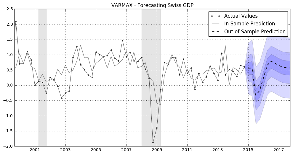
Comments You need to have a GitHub Account to comment!
Post comment